马尔科夫随机场

Markov Random Fields

Theory

We can optionally use prior information by applying a Hidden Markov Random Field (HMRF) model. Using this model we introduce spatial constraints based on neighbouring voxels of a 3x3x3 cube. The center voxel has 26 neighbours and we can calculate MRF energy by counting the number of neighbours. Neighboring voxels are expected to have the same class labels. The prior probability of the class and the likelihood probability of the observation is combined to estimate the Maximum a posteriori (MAP). Prior probability can be weighted between 0 (no HMRF) and 1 (maximum HMRF for very noisy data) to cover different levels of noise. Parts of this version are based on an implementation of a Gaussian Hidden Markov Random Field (GHMRF) approach byMeritxell Bach Cuadra et al. (2005).

The idea is to remove isolated voxels of one tissue class which are unlikely to be member of this tissue type. It also closes holes in a cluster of connected voxels of one tissue type. In the resulting segmentation the noise level will be minimized.

Depending on your scanner and the used MR sequence your T1-images will contain at least 3% noise level. Hence, I would recommend for most images a medium HMRF weighting of 0.3. If your images are affected by more noise level you can choose a larger HMRF weighting.

The resulting files are indicated by the term “_HMRF” at the end of the filename.

MRF energy

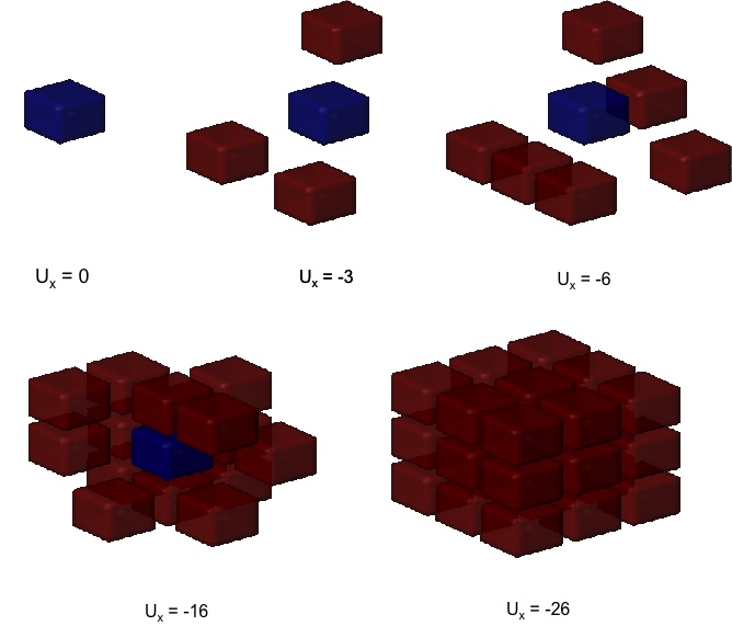
MRF energy Ux is caclulated by counting the number of neigbouring voxels of one tissue class in a 3x3x3 cube. From upper left to lower right there are different configurations shown from Ux=0 (no neighbours) up to Ux=-26 (maximum number of 26 neighbours)

Use of MRF prior probability

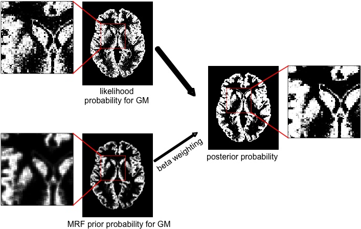
Based on the MRF energy we calculate MRF prior probabilities for each tissue class. This prior information is combined with the likelihood probability from the segmentation step to a joint posterior probability. The amount to which this prior information is used can be controlled with a weighting factor beta

Effect of noise reduction

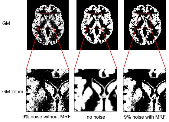
In the center we can see the result of gray matter segmentation of the ground truth image from the brainweb database without any noise. The lower panel shows an enlarged view to demonstrate the segmentation quality. On the left the result with a noise level of 9% is shown quality of the image is degraded. On the right side we can see the result with MRF application and the amount of noise in the segmentation is diminished.

Comparison with segmentation without MRF approach

To validate the effect of applying MRF we use a ground truth image from the brainweb database with varying noise levels of 1..9%. Segmentation accuracy for gray matter is calculated by using a kappa coefficent. A kappa coefficient of 1 means that there is perfect overlap between the ground truth reference and the segmented image. Without application of MRF the kappa coefficient is much lower for larger noise levels because of the decreased signal-to-noise ratio. By applying the MRF we obtain larger kappa coefficients for noise levels >3-5%. The usual noise level in a standard T1 image is around 3% or higher, hence the application of MRF helps in obtaining more accurate segmentations.

Alexander Ovsov translated this site to Romanian language for Web Geek Science.

来源：http://dbm.neuro.uni-jena.de/vbm/markov-random-fields/