Heaviside step function 阶跃函数

来源：互联网发布：淘宝自定义分类模板编辑：程序博客网时间：2024/05/23 01:13

Heaviside step function 阶跃函数

Heaviside step functionFrom Wikipedia, the free encyclopedia Jump to: navigation, search

The Heaviside step function, using the half-maximum convention

The Heaviside step function, H, also called the unit step function, is a discontinuous function whose value is zero for negative argument and one for positive argument. It seldom matters what value is used for H(0), since H is mostly used as a distribution. Some common choices can be seen below.

The function is used in the mathematics of control theory and signal processing to represent a signal that switches on at a specified time and stays switched on indefinitely. It was named after the English polymath Oliver Heaviside.

It is the cumulative distribution function of a random variable which is almost surely 0. (See constant random variable.)

The Heaviside function is the integral of the Dirac delta function: H′ = δ. This is sometimes written as

$H(x) = \int_{-\infty}^x { \delta(t)} \mathrm{d}t$

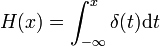
although this expansion may not hold (or even make sense) for x = 0, depending on which formalism one uses to give meaning to integrals involving δ.

Contents []

1 Discrete form
2 Analytic approximations
3 Representations
4 H(0)
5 Antiderivative and derivative
6 Fourier transform
7 See also
8 References

[edit] Discrete form

We can also define an alternative form of the unit step as a function of a discrete variable n:

$H[n]=\begin{cases} 0, & n < 0 \\ 1, & n \ge 0 \end{cases}$

where n is an integer.

The discrete-time unit impulse is the first difference of the discrete-time step

$\delta\left[ n \right] = H[n] - H[n-1].$

This function is the cumulative summation of the Kronecker delta:

$H[n] = \sum_{k=-\infty}^{n} \delta[k] \,$

where

$\delta[k] = \delta_{k,0} \,$

is the discrete unit impulse function.

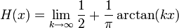
[edit] Analytic approximations

For a smooth approximation to the step function, one can use the logistic function

$H(x) \approx \frac{1}{2} + \frac{1}{2}\tanh(kx) = \frac{1}{1+\mathrm{e}^{-2kx}}$ ,

where a larger k corresponds to a sharper transition at x = 0. If we take H(0) = ½, equality holds in the limit:

$H(x)=\lim_{k \rightarrow \infty}\frac{1}{2}(1+\tanh kx)=\lim_{k \rightarrow \infty}\frac{1}{1+\mathrm{e}^{-2kx}}.$

There are many other smooth, analytic approximations to the step function.[1] They include:

$H(x) = \lim_{k \rightarrow \infty} \frac{1}{2} + \frac{1}{\pi}\arctan(kx) \$

$H(x) = \lim_{k \rightarrow \infty} \frac{1}{2} + \frac{1}{2}\operatorname{erf}(kx). \$

While these approximations converge pointwise towards the step function, the implied distributions do not strictly converge towards the delta distribution. In particular, the measurable set

$\bigcup_{n=0}^{\infty}\left[ 2^{-2n};2^{-2n+1}\right]$

has measure zero in the delta distribution, but its measure under each smooth approximation family becomes larger with increasing k.

[edit] Representations

Often an integral representation of the Heaviside step function is useful:

$H(x)=\lim_{ \epsilon \to 0^+} -{1\over 2\pi \mathrm{i}}\int_{-\infty}^\infty {1 \over \tau+\mathrm{i}\epsilon} \mathrm{e}^{-\mathrm{i} x \tau} \mathrm{d}\tau =\lim_{ \epsilon \to 0^+} {1\over 2\pi \mathrm{i}}\int_{-\infty}^\infty {1 \over \tau-\mathrm{i}\epsilon} \mathrm{e}^{\mathrm{i} x \tau} \mathrm{d}\tau.$

[edit] H(0)

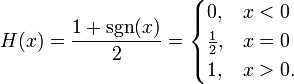
The value of the function at 0 can be defined as H(0) = 0, H(0) = ½ or H(0) = 1. H(0) = ½ is the most consistent choice used, since it maximizes the symmetry of the function and becomes completely consistent with the sign function. This makes for a more general definition:

$H(x) = \frac{1+\sgn(x)}{2} =\begin{cases} 0, & x < 0\\ \frac{1}{2}, & x = 0\\ 1, & x > 0.\end{cases}$

To remove the ambiguity of which value to use for H(0), a subscript specifying the value may be used:

$H_a(x) =\begin{cases} 0, & x < 0\\ a, & x = 0\\ 1, & x > 0.\end{cases}$

[edit] Antiderivative and derivative

The ramp function is the antiderivative of the Heaviside step function: 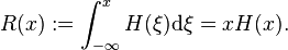$R(x) := \int_{-\infty}^{x} H(\xi)\mathrm{d}\xi = x H(x).$

The derivative of the Heaviside step function is the Dirac delta function: dH(x) / dx = δ(x).

[edit] Fourier transform

The Fourier transform of the Heaviside step function is a distribution. Using one choice of constants for the definition of the Fourier transform we have

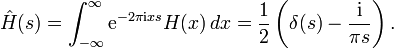
$\hat{H}(s) = \int^{\infty}_{-\infty} \mathrm{e}^{-2\pi\mathrm{i} x s} H(x)\, dx = \frac{1}{2} \left( \delta(s) - \frac{ \mathrm{i}}{\pi s} \right).$

Here the $\frac{1}{s}$ term must be interpreted as a distribution that takes a test function φ to the Cauchy principal value of $\int^{\infty}_{-\infty} \phi(x)/x\, dx.$

[edit] See also

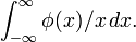
Rectangular function
Step response
Sign function
Negative and non-negative numbers
Laplace transform
Iverson bracket

[edit] References

^ Eric W. Weisstein, Heaviside Step Function at MathWorld.

Retrieved from "http://en.wikipedia.org/wiki/Heaviside_step_function"Categories: Elementary special functions | Generalized functions

#数学方法&公式推导