UFLDL Tutorial_Vectorized implementation

Vectorization

When working with learning algorithms, having a faster piece of code often means that you'll make progress faster on your project. For example, if your learning algorithm takes 20 minutes to run to completion, that means you can "try" up to 3 new ideas per hour. But if your code takes 20 hours to run, that means you can "try" only one idea a day, since that's how long you have to wait to get feedback from your program. In this latter case, if you can speed up your code so that it takes only 10 hours to run, that can literally double your personal productivity!

Vectorization refers to a powerful way to speed up your algorithms. Numerical computing and parallel computing researchers have put decades of work into making certain numerical operations (such as matrix-matrix multiplication, matrix-matrix addition, matrix-vector multiplication) fast. The idea of vectorization is that we would like to express our learning algorithms in terms of these highly optimized operations.

For example, if  and  are vectors and you need to compute , you can implement (in Matlab):

z = 0;for i=1:(n+1),  z = z + theta(i) * x(i);end;

or you can more simply implement

z = theta' * x;

The second piece of code is not only simpler, but it will also run much faster.

More generally, a good rule-of-thumb for coding Matlab/Octave is:

Whenever possible, avoid using explicit for-loops in your code.

In particular, the first code example used an explicit for loop. By implementing the same functionality without the for loop, we sped it up significantly. A large part of vectorizing our Matlab/Octave code will focus on getting rid of for loops, since this lets Matlab/Octave extract more parallelism from your code, while also incurring less computational overhead from the interpreter.

In terms of a strategy for writing your code, initially you may find that vectorized code is harder to write, read, and/or debug, and that there may be a tradeoff in ease of programming/debugging vs. running time. Thus, for your first few programs, you might choose to first implement your algorithm without too many vectorization tricks, and verify that it is working correctly (perhaps by running on a small problem). Then only after it is working, you can vectorize your code one piece at a time, pausing after each piece to verify that your code is still computing the same result as before. At the end, you'll then hopefully have a correct, debugged, and vectorized/efficient piece of code.

After you become familiar with the most common vectorization methods and tricks, you'll find that it usually isn't much effort to vectorize your code. Doing so will make your code run much faster and, in some cases, simplify it too.

Logistic Regression Vectorization Example

Consider training a logistic regression model using batch gradient ascent. Suppose our hypothesis is

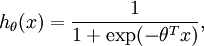
where (following the notational convention from the OpenClassroom videos and from CS229) we let , so that  and , and  is our intercept term. We have a training set  of  examples, and the batch gradient ascent update rule is 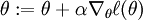, where  is the log likelihood and  is its derivative.

[Note: Most of the notation below follows that defined in the OpenClassroom videos or in the class CS229: Machine Learning. For details, see either the OpenClassroom videos or Lecture Notes #1 of http://cs229.stanford.edu/ .]

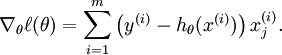
We thus need to compute the gradient:

Suppose that the Matlab/Octave variable x is a matrix containing the training inputs, so that x(:,i) is the -th training example , and x(j,i) is . Further, suppose the Matlab/Octave variable y is a row vector of the labels in the training set, so that the variable y(i) is . (Here we differ from the OpenClassroom/CS229 notation. Specifically, in the matrix-valued x we stack the training inputs in columns rather than in rows; and y is a row vector rather than a column vector.)

Here's truly horrible, extremely slow, implementation of the gradient computation:

% Implementation 1grad = zeros(n+1,1);for i=1:m,  h = sigmoid(theta'*x(:,i));  temp = y(i) - h;   for j=1:n+1,    grad(j) = grad(j) + temp * x(j,i);   end;end;

The two nested for-loops makes this very slow. Here's a more typical implementation, that partially vectorizes the algorithm and gets better performance:

% Implementation 2 grad = zeros(n+1,1);for i=1:m,  grad = grad + (y(i) - sigmoid(theta'*x(:,i)))* x(:,i);end;

However, it turns out to be possible to even further vectorize this. If we can get rid of the for-loop, we can significantly speed up the implementation. In particular, suppose b is a column vector, and A is a matrix. Consider the following ways of computing A * b:

% Slow implementation of matrix-vector multiplygrad = zeros(n+1,1);for i=1:m,  grad = grad + b(i) * A(:,i);  % more commonly written A(:,i)*b(i)end; % Fast implementation of matrix-vector multiplygrad = A*b;

We recognize that Implementation 2 of our gradient descent calculation above is using the slow version with a for-loop, with b(i)playing the role of (y(i) - sigmoid(theta'*x(:,i))), and A playing the role of x. We can derive a fast implementation as follows:

% Implementation 3grad = x * (y- sigmoid(theta'*x))';

Here, we assume that the Matlab/Octave sigmoid(z) takes as input a vector z, applies the sigmoid function component-wise to the input, and returns the result. The output of sigmoid(z) is therefore itself also a vector, of the same dimension as the input z

When the training set is large, this final implementation takes the greatest advantage of Matlab/Octave's highly optimized numerical linear algebra libraries to carry out the matrix-vector operations, and so this is far more efficient than the earlier implementations.

Coming up with vectorized implementations isn't always easy, and sometimes requires careful thought. But as you gain familiarity with vectorized operations, you'll find that there are design patterns (i.e., a small number of ways of vectorizing) that apply to many different pieces of code.

Neural Network Vectorization

In this section, we derive a vectorized version of our neural network. In our earlier description of Neural Networks, we had already given a partially vectorized implementation, that is quite efficient if we are working with only a single example at a time. We now describe how to implement the algorithm so that it simultaneously processes multiple training examples. Specifically, we will do this for the forward propagation and backpropagation steps, as well as for learning a sparse set of features.

Forward propagation

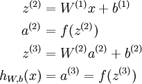
Consider a 3 layer neural network (with one input, one hidden, and one output layer), and suppose x is a column vector containing a single training example . Then the forward propagation step is given by:

This is a fairly efficient implementation for a single example. If we have m examples, then we would wrap a for loop around this.

Concretely, following the Logistic Regression Vectorization Example, let the Matlab/Octave variable x be a matrix containing the training inputs, so that x(:,i) is the -th training example. We can then implement forward propagation as:

 % Unvectorized implementationfor i=1:m,   z2 = W1 * x(:,i) + b1;  a2 = f(z2);  z3 = W2 * a2 + b2;  h(:,i) = f(z3);end;

Can we get rid of the for loop? For many algorithms, we will represent intermediate stages of computation via vectors. For example,z2, a2, and z3 here are all column vectors that're used to compute the activations of the hidden and output layers. In order to take better advantage of parallelism and efficient matrix operations, we would like to have our algorithm operate simultaneously on many training examples. Let us temporarily ignore b1 and b2 (say, set them to zero for now). We can then implement the following:

% Vectorized implementation (ignoring b1, b2)z2 = W1 * x;a2 = f(z2);z3 = W2 * a2;h = f(z3)

In this implementation, z2, a2, and z3 are all matrices, with one column per training example. A common design pattern in vectorizing across training examples is that whereas previously we had a column vector (such as z2) per training example, we can often instead try to compute a matrix so that all of these column vectors are stacked together to form a matrix. Concretely, in this example, a2 becomes a s₂ by m matrix (where s₂ is the number of units in layer 2 of the network, and m is the number of training examples). And, the i-th column of a2 contains the activations of the hidden units (layer 2 of the network) when the i-th training example x(:,i) is input to the network.

In the implementation above, we have assumed that the activation function f(z) takes as input a matrix z, and applies the activation function component-wise to the input. Note that your implementation of f(z) should use Matlab/Octave's matrix operations as much as possible, and avoid for loops as well. We illustrate this below, assuming that f(z) is the sigmoid activation function:

% Inefficient, unvectorized implementation of the activation functionfunction output = unvectorized_f(z)output = zeros(size(z))for i=1:size(z,1),   for j=1:size(z,2),    output(i,j) = 1/(1+exp(-z(i,j)));  end; end;end % Efficient, vectorized implementation of the activation functionfunction output = vectorized_f(z)output = 1./(1+exp(-z));     % "./" is Matlab/Octave's element-wise division operator. end

Finally, our vectorized implementation of forward propagation above had ignored b1 and b2. To incorporate those back in, we will use Matlab/Octave's built-in repmat function. We have:

% Vectorized implementation of forward propagationz2 = W1 * x + repmat(b1,1,m);a2 = f(z2);z3 = W2 * a2 + repmat(b2,1,m);h = f(z3)

The result of repmat(b1,1,m) is a matrix formed by taking the column vector b1 and stacking m copies of them in columns as follows

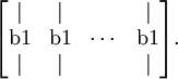
This forms a s₂ by m matrix. Thus, the result of adding this to W1 * x is that each column of the matrix gets b1 added to it, as desired. See Matlab/Octave's documentation (type "help repmat") for more information. As a Matlab/Octave built-in function, repmat is very efficient as well, and runs much faster than if you were to implement the same thing yourself using a for loop.

Backpropagation

We now describe the main ideas behind vectorizing backpropagation. Before reading this section, we strongly encourage you to carefully step through all the forward propagation code examples above to make sure you fully understand them. In this text, we'll only sketch the details of how to vectorize backpropagation, and leave you to derive the details in the Vectorization exercise.

We are in a supervised learning setting, so that we have a training set  of m training examples. (For the autoencoder, we simply set y⁽ⁱ⁾ = x⁽ⁱ⁾, but our derivation here will consider this more general setting.)

Suppose we have s₃ dimensional outputs, so that our target labels are . In our Matlab/Octave datastructure, we will stack these in columns to form a Matlab/Octave variable y, so that the i-th column y(:,i) is y⁽ⁱ⁾.

We now want to compute the gradient terms 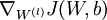 and . Consider the first of these terms. Following our earlier description of the Backpropagation Algorithm, we had that for a single training example (x,y), we can compute the derivatives as

Here,  denotes element-wise product. For simplicity, our description here will ignore the derivatives with respect to b^(l), though your implementation of backpropagation will have to compute those derivatives too.

Suppose we have already implemented the vectorized forward propagation method, so that the matrix-valued z2, a2, z3 and h are computed as described above. We can then implement an unvectorized version of backpropagation as follows:

gradW1 = zeros(size(W1));gradW2 = zeros(size(W2)); for i=1:m,  delta3 = -(y(:,i) - h(:,i)) .* fprime(z3(:,i));   delta2 = W2'*delta3(:,i) .* fprime(z2(:,i));   gradW2 = gradW2 + delta3*a2(:,i)';  gradW1 = gradW1 + delta2*a1(:,i)'; end;

This implementation has a for loop. We would like to come up with an implementation that simultaneously performs backpropagation on all the examples, and eliminates this for loop.

To do so, we will replace the vectors delta3 and delta2 with matrices, where one column of each matrix corresponds to each training example. We will also implement a function fprime(z) that takes as input a matrix z, and applies  element-wise. Each of the four lines of Matlab in the for loop above can then be vectorized and replaced with a single line of Matlab code (without a surroundingfor loop).

In the Vectorization exercise, we ask you to derive the vectorized version of this algorithm by yourself. If you are able to do it from this description, we strongly encourage you to do so. Here also are some Backpropagation vectorization hints; however, we encourage you to try to carry out the vectorization yourself without looking at the hints.

Sparse autoencoder

The sparse autoencoder neural network has an additional sparsity penalty that constrains neurons' average firing rate to be close to some target activation ρ. When performing backpropagation on a single training example, we had taken into the account the sparsity penalty by computing the following:

In the unvectorized case, this was computed as:

% Sparsity Penalty Deltasparsity_delta = - rho ./ rho_hat + (1 - rho) ./ (1 - rho_hat);for i=1:m,  ...  delta2 = (W2'*delta3(:,i) + beta*sparsity_delta).* fprime(z2(:,i));   ...end;

The code above still had a for loop over the training set, and delta2 was a column vector.

In contrast, recall that in the vectorized case, delta2 is now a matrix with m columns corresponding to the m training examples. Now, notice that the sparsity_delta term is the same regardless of what training example we are processing. This suggests that vectorizing the computation above can be done by simply adding the same value to each column when constructing the delta2 matrix. Thus, to vectorize the above computation, we can simply add sparsity_delta (e.g., using repmat) to each column of delta2.

Exercise:Vectorization

Contents

 [hide]

• 1 Vectorization
  • 1.1 Support Code/Data
  • 1.2 Step 1: Vectorize your Sparse Autoencoder Implementation
  • 1.3 Step 2: Learn features for handwritten digits

Vectorization

In the previous problem set, we implemented a sparse autoencoder for patches taken from natural images. In this problem set, you will vectorize your code to make it run much faster, and further adapt your sparse autoencoder to work on images of handwritten digits. Your network for learning from handwritten digits will be much larger than the one you'd trained on the natural images, and so using the original implementation would have been painfully slow. But with a vectorized implementation of the autoencoder, you will be able to get this to run in a reasonable amount of computation time.

Support Code/Data

The following additional files are required for this exercise:

• MNIST Dataset (Training Images)
• MNIST Dataset (Training Labels)
• Support functions for loading MNIST in Matlab

Step 1: Vectorize your Sparse Autoencoder Implementation

Using the ideas from Vectorization and Neural Network Vectorization, vectorize your implementation of sparseAutoencoderCost.m. In our implementation, we were able to remove all for-loops with the use of matrix operations and repmat. (If you want to play with more advanced vectorization ideas, also type help bsxfun. The bsxfun function provides an alternative to repmat for some of the vectorization steps, but is not necessary for this exercise). A vectorized version of our sparse autoencoder code ran in under one minute on a fast computer (for learning 25 features from 10000 8x8 image patches).

(Note that you do not need to vectorize the code in the other files.)

Step 2: Learn features for handwritten digits

Now that you have vectorized the code, it is easy to learn larger sets of features on medium sized images. In this part of the exercise, you will use your sparse autoencoder to learn features for handwritten digits from the MNIST dataset.

The MNIST data is available at [1]. Download the file train-images-idx3-ubyte.gz and decompress it. After obtaining the source images, you should use helper functions that we provide to load the data into Matlab as matrices. While the helper functions that we provide will load both the input examples x and the class labels y, for this assignment, you will only need the input examples xsince the sparse autoencoder is an unsupervised learning algorithm. (In a later assignment, we will use the labels y as well.)

The following set of parameters worked well for us to learn good features on the MNIST dataset:

visibleSize = 28*28hiddenSize = 196sparsityParam = 0.1lambda = 3e-3beta = 3patches = first 10000 images from the MNIST dataset

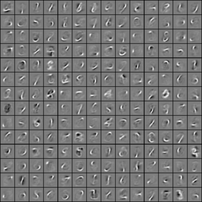
After 400 iterations of updates using minFunc, your autoencoder should have learned features that resemble pen strokes. In other words, this has learned to represent handwritten characters in terms of what pen strokes appear in an image. Our implementation takes around 15-20 minutes on a fast machine. Visualized, the features should look like the following image:

If your parameters are improperly tuned, or if your implementation of the autoencoder is buggy, you may get one of the following images instead:

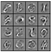
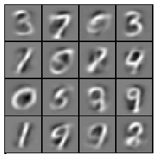
If your image looks like one of the above images, check your code and parameters again. Learning these features are a prelude to the later exercises, where we shall see how they will be useful for classification.