UFLDL Tutorial_Linear Decoders with Autoencoders

Linear Decoders

Sparse Autoencoder Recap

In the sparse autoencoder, we had 3 layers of neurons: an input layer, a hidden layer and an output layer. In our previous description of autoencoders (and of neural networks), every neuron in the neural network used the same activation function. In these notes, we describe a modified version of the autoencoder in which some of the neurons use a different activation function. This will result in a model that is sometimes simpler to apply, and can also be more robust to variations in the parameters.

Recall that each neuron (in the output layer) computed the following:

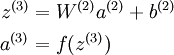
where a⁽³⁾ is the output. In the autoencoder, a⁽³⁾ is our approximate reconstruction of the input x = a⁽¹⁾.

Because we used a sigmoid activation function for f(z⁽³⁾), we needed to constrain or scale the inputs to be in the range [0,1], since the sigmoid function outputs numbers in the range [0,1]. While some datasets like MNIST fit well with this scaling of the output, this can sometimes be awkward to satisfy. For example, if one uses PCA whitening, the input is no longer constrained to[0,1] and it's not clear what the best way is to scale the data to ensure it fits into the constrained range.

Linear Decoder

One easy fix for this problem is to set a⁽³⁾ = z⁽³⁾. Formally, this is achieved by having the output nodes use an activation function that's the identity function f(z) = z, so that a⁽³⁾ = f(z⁽³⁾) = z⁽³⁾. This particular activation function  is called thelinear activation function (though perhaps "identity activation function" would have been a better name). Note however that in the hidden layer of the network, we still use a sigmoid (or tanh) activation function, so that the hidden unit activations are given by (say) 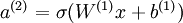, where  is the sigmoid function, x is the input, and W⁽¹⁾ and b⁽¹⁾ are the weight and bias terms for the hidden units. It is only in the output layer that we use the linear activation function.

An autoencoder in this configuration--with a sigmoid (or tanh) hidden layer and a linear output layer--is called a linear decoder. In this model, we have . Because the output  is a now linear function of the hidden unit activations, by varying W⁽²⁾, each output unit a⁽³⁾ can be made to produce values greater than 1 or less than 0 as well. This allows us to train the sparse autoencoder real-valued inputs without needing to pre-scale every example to a specific range.

Since we have changed the activation function of the output units, the gradients of the output units also change. Recall that for each output unit, we had set set the error terms as follows:

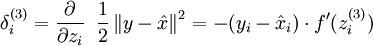
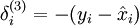
where y = x is the desired output,  is the output of our autoencoder, and  is our activation function. Because in the output layer we now have f(z) = z, that implies f'(z) = 1 and thus the above now simplifies to:

Of course, when using backpropagation to compute the error terms for the hidden layer:

Because the hidden layer is using a sigmoid (or tanh) activation f, in the equation above  should still be the derivative of the sigmoid (or tanh) function.

Contents

• CS294A/CS294W Linear Decoder Exercise
• STEP 0: Initialization
• STEP 1: Create and modify sparseAutoencoderLinearCost.m to use a linear decoder,
• STEP 2: Learn features on small patches
• STEP 2a: Load patches
• STEP 2b: Apply preprocessing
• STEP 2c: Learn features
• STEP 2d: Visualize learned features

CS294A/CS294W Linear Decoder Exercise

%  Instructions%  ------------%%  This file contains code that helps you get started on the%  linear decoder exericse. For this exercise, you will only need to modify%  the code in sparseAutoencoderLinearCost.m. You will not need to modify%  any code in this file.%%======================================================================

STEP 0: Initialization

Here we initialize some parameters used for the exercise.

imageChannels = 3;     % number of channels (rgb, so 3)patchDim   = 8;          % patch dimensionnumPatches = 100000;   % number of patchesvisibleSize = patchDim * patchDim * imageChannels;  % number of input unitsoutputSize  = visibleSize;   % number of output unitshiddenSize  = 400;           % number of hidden units %中间的隐含层还变多了sparsityParam = 0.035; % desired average activation of the hidden units.lambda = 3e-3;         % weight decay parameterbeta = 5;              % weight of sparsity penalty termepsilon = 0.1;           % epsilon for ZCA whitening%%======================================================================

STEP 1: Create and modify sparseAutoencoderLinearCost.m to use a linear decoder,

        and check gradientsYou should copy sparseAutoencoderCost.m from your earlier exerciseand rename it to sparseAutoencoderLinearCost.m.Then you need to rename the function from sparseAutoencoderCost tosparseAutoencoderLinearCost, and modify it so that the sparse autoencoderuses a linear decoder instead. Once that is done, you should checkyour gradients to verify that they are correct.

% NOTE: Modify sparseAutoencoderCost first!% To speed up gradient checking, we will use a reduced network and some% dummy patchesdebugHiddenSize = 5;debugvisibleSize = 8;patches = rand([8 10]);%随机产生10个样本，每个样本为一个8维的列向量，元素值为0~1theta = initializeParameters(debugHiddenSize, debugvisibleSize);[cost, grad] = sparseAutoencoderLinearCost(theta, debugvisibleSize, debugHiddenSize, ...                                           lambda, sparsityParam, beta, ...                                           patches);% Check gradientsnumGrad = computeNumericalGradient( @(x) sparseAutoencoderLinearCost(x, debugvisibleSize, debugHiddenSize, ...                                                  lambda, sparsityParam, beta, ...                                                  patches), theta);% Use this to visually compare the gradients side by sidedisp([numGrad grad]);diff = norm(numGrad-grad)/norm(numGrad+grad);% Should be small. In our implementation, these values are usually less than 1e-9.disp(diff);assert(diff < 1e-9, 'Difference too large. Check your gradient computation again');% NOTE: Once your gradients check out, you should run step 0 again to%       reinitialize the parameters%}%%======================================================================

STEP 2: Learn features on small patches

In this step, you will use your sparse autoencoder (which now uses alinear decoder) to learn features on small patches sampled from relatedimages.

STEP 2a: Load patches

In this step, we load 100k patches sampled from the STL10 dataset andvisualize them. Note that these patches have been scaled to [0,1]

load stlSampledPatches.matdisplayColorNetwork(patches(:, 1:100));patches=patches(:,1:1000); %取1000个样本做实验

STEP 2b: Apply preprocessing

In this sub-step, we preprocess the sampled patches, in particular,ZCA whitening them.

In a later exercise on convolution and pooling, you will need to replicateexactly the preprocessing steps you apply to these patches beforeusing the autoencoder to learn features on them. Hence, we will save theZCA whitening and mean image matrices together with the learned featureslater on.

% Subtract mean patch (hence zeroing the mean of the patches)meanPatch = mean(patches, 2);  %注意这里减掉的是每一维属性的均值，为什么会和其它的不同呢？patches = bsxfun(@minus, patches, meanPatch);%每一维都均值化% Apply ZCA whiteningsigma = patches * patches' / numPatches;[u, s, v] = svd(sigma);ZCAWhite = u * diag(1 ./ sqrt(diag(s) + epsilon)) * u';%求出ZCAWhitening矩阵patches = ZCAWhite * patches;figuredisplayColorNetwork(patches(:, 1:100));

STEP 2c: Learn features

You will now use your sparse autoencoder (with linear decoder) to learnfeatures on the preprocessed patches. This should take around 45 minutes.

theta = initializeParameters(hiddenSize, visibleSize);% Use minFunc to minimize the functionaddpath minFunc/options = struct;options.Method = 'cg';options.maxIter = 400;options.display = 'on';[optTheta, cost] = minFunc( @(p) sparseAutoencoderLinearCost(p, ...                                   visibleSize, hiddenSize, ...                                   lambda, sparsityParam, ...                                   beta, patches), ...                              theta, options);%注意它的参数% Save the learned features and the preprocessing matrices for use in% the later exercise on convolution and poolingfprintf('Saving learned features and preprocessing matrices...\n');save('STL10Features.mat', 'optTheta', 'ZCAWhite', 'meanPatch');fprintf('Saved\n');

STEP 2d: Visualize learned features

W = reshape(optTheta(1:visibleSize * hiddenSize), hiddenSize, visibleSize);b = optTheta(2*hiddenSize*visibleSize+1:2*hiddenSize*visibleSize+hiddenSize);figure;%这里为什么要用(W*ZCAWhite)'呢？首先，使用W*ZCAWhite是因为每个样本x输入网络，%其输出等价于W*ZCAWhite*x；另外，由于W*ZCAWhite的每一行才是一个隐含节点的变换值%而displayColorNetwork函数是把每一列显示一个小图像块的，所以需要对其转置。displayColorNetwork( (W*ZCAWhite)');

Contents

• ---------- YOUR CODE HERE --------------------------------------

function [cost,grad] = sparseAutoencoderLinearCost(theta, visibleSize, hiddenSize, ...                                                            lambda, sparsityParam, beta, data)

% -------------------- YOUR CODE HERE --------------------% Instructions:%   Copy sparseAutoencoderCost in sparseAutoencoderCost.m from your%   earlier exercise onto this file, renaming the function to%   sparseAutoencoderLinearCost, and changing the autoencoder to use a%   linear decoder.% -------------------- YOUR CODE HERE --------------------% The input theta is a vector because minFunc only deal with vectors. In% this step, we will convert theta to matrix format such that they follow% the notation in the lecture notes.W1 = reshape(theta(1:hiddenSize*visibleSize), hiddenSize, visibleSize);W2 = reshape(theta(hiddenSize*visibleSize+1:2*hiddenSize*visibleSize), visibleSize, hiddenSize);b1 = theta(2*hiddenSize*visibleSize+1:2*hiddenSize*visibleSize+hiddenSize);b2 = theta(2*hiddenSize*visibleSize+hiddenSize+1:end);% Loss and gradient variables (your code needs to compute these values)m = size(data, 2);%样本点的个数

---------- YOUR CODE HERE --------------------------------------

Instructions: Compute the loss for the Sparse Autoencoder and gradients              W1grad, W2grad, b1grad, b2grad

Hint: 1) data(:,i) is the i-th example      2) your computation of loss and gradients should match the size      above for loss, W1grad, W2grad, b1grad, b2grad

% z2 = W1 * x + b1% a2 = f(z2)% z3 = W2 * a2 + b2% h_Wb = a3 = f(z3)z2 = W1 * data + repmat(b1, [1, m]);a2 = sigmoid(z2);z3 = W2 * a2 + repmat(b2, [1, m]);a3 = z3;rhohats = mean(a2,2);rho = sparsityParam;KLsum = sum(rho * log(rho ./ rhohats) + (1-rho) * log((1-rho) ./ (1-rhohats)));squares = (a3 - data).^2;squared_err_J = (1/2) * (1/m) * sum(squares(:));weight_decay_J = (lambda/2) * (sum(W1(:).^2) + sum(W2(:).^2));sparsity_J = beta * KLsum;cost = squared_err_J + weight_decay_J + sparsity_J;%损失函数值% delta3 = -(data - a3) .* fprime(z3);% but fprime(z3) = a3 * (1-a3)delta3 = -(data - a3);beta_term = beta * (- rho ./ rhohats + (1-rho) ./ (1-rhohats));delta2 = ((W2' * delta3) + repmat(beta_term, [1,m]) ) .* a2 .* (1-a2);W2grad = (1/m) * delta3 * a2' + lambda * W2;b2grad = (1/m) * sum(delta3, 2);W1grad = (1/m) * delta2 * data' + lambda * W1;b1grad = (1/m) * sum(delta2, 2);%-------------------------------------------------------------------% Convert weights and bias gradients to a compressed form% This step will concatenate and flatten all your gradients to a vector% which can be used in the optimization method.grad = [W1grad(:) ; W2grad(:) ; b1grad(:) ; b2grad(:)];

end%-------------------------------------------------------------------% We are giving you the sigmoid function, you may find this function% useful in your computation of the loss and the gradients.function sigm = sigmoid(x)    sigm = 1 ./ (1 + exp(-x));end

function displayColorNetwork(A)% display receptive field(s) or basis vector(s) for image patches%% A         the basis, with patches as column vectors% In case the midpoint is not set at 0, we shift it dynamicallyif min(A(:)) >= 0    A = A - mean(A(:));endcols = round(sqrt(size(A, 2)));channel_size = size(A,1) / 3;dim = sqrt(channel_size);dimp = dim+1;rows = ceil(size(A,2)/cols);B = A(1:channel_size,:);C = A(channel_size+1:channel_size*2,:);D = A(2*channel_size+1:channel_size*3,:);B=B./(ones(size(B,1),1)*max(abs(B)));C=C./(ones(size(C,1),1)*max(abs(C)));D=D./(ones(size(D,1),1)*max(abs(D)));% Initialization of the imageI = ones(dim*rows+rows-1,dim*cols+cols-1,3);%Transfer features to this image matrixfor i=0:rows-1  for j=0:cols-1    if i*cols+j+1 > size(B, 2)        break    end    % This sets the patch    I(i*dimp+1:i*dimp+dim,j*dimp+1:j*dimp+dim,1) = ...         reshape(B(:,i*cols+j+1),[dim dim]);    I(i*dimp+1:i*dimp+dim,j*dimp+1:j*dimp+dim,2) = ...         reshape(C(:,i*cols+j+1),[dim dim]);    I(i*dimp+1:i*dimp+dim,j*dimp+1:j*dimp+dim,3) = ...         reshape(D(:,i*cols+j+1),[dim dim]);  endendI = I + 1;I = I / 2;imagesc(I);axis equalaxis offend