UFLDL Tutorial_Sparse Coding

来源：互联网发布：js浮点数精度问题编辑：程序博客网时间：2024/05/21 21:35

Sparse Coding

Sparse coding is a class of unsupervised methods for learning sets of over-complete bases to represent data efficiently. The aim of sparse coding is to find a set of basis vectors $\mathbf{\phi}_i$ such that we can represent an input vector $\mathbf{x}$ as a linear combination of these basis vectors:

$\begin{align}\mathbf{x} = \sum_{i=1}^k a_i \mathbf{\phi}_{i} \end{align}$

While techniques such as Principal Component Analysis (PCA) allow us to learn a complete set of basis vectors efficiently, we wish to learn an over-complete set of basis vectors to represent input vectors $\mathbf{x}\in\mathbb{R}^n$ (i.e. such that $k > n$ ). The advantage of having an over-complete basis is that our basis vectors are better able to capture structures and patterns inherent in the input data. However, with an over-complete basis, the coefficients $a i$ are no longer uniquely determined by the input vector $\mathbf{x}$ . Therefore, in sparse coding, we introduce the additional criterion of sparsity to resolve the degeneracy introduced by over-completeness.

Here, we define sparsity as having few non-zero components or having few components not close to zero. The requirement that our coefficients $a i$ be sparse means that given a input vector, we would like as few of our coefficients to be far from zero as possible. The choice of sparsity as a desired characteristic of our representation of the input data can be motivated by the observation that most sensory data such as natural images may be described as the superposition of a small number of atomic elements such as surfaces or edges. Other justifications such as comparisons to the properties of the primary visual cortex have also been advanced.

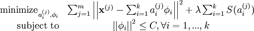
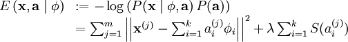
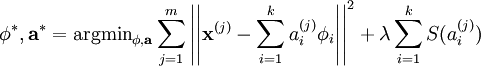
We define the sparse coding cost function on a set of $m$ input vectors as

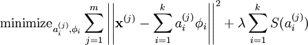
$\begin{align}\text{minimize}_{a^{(j)}_i,\mathbf{\phi}_{i}} \sum_{j=1}^{m} \left|\left| \mathbf{x}^{(j)} - \sum_{i=1}^k a^{(j)}_i \mathbf{\phi}_{i}\right|\right|^{2} + \lambda \sum_{i=1}^{k}S(a^{(j)}_i)\end{align}$

where $S (.)$ is a sparsity cost function which penalizes $a i$ for being far from zero. We can interpret the first term of the sparse coding objective as a reconstruction term which tries to force the algorithm to provide a good representation of $\mathbf{x}$ and the second term as a sparsity penalty which forces our representation of $\mathbf{x}$ to be sparse. The constant $λ$ is a scaling constant to determine the relative importance of these two contributions.

Although the most direct measure of sparsity is the " $L 0$ " norm ( $S(a_i) = \mathbf{1}(|a_i|>0)$ ), it is non-differentiable and difficult to optimize in general. In practice, common choices for the sparsity cost $S (.)$ are the $L 1$ penalty $S(a_i)=\left|a_i\right|_1$ and the log penalty $S(a_i)=\log(1+a_i^2)$ .

In addition, it is also possible to make the sparsity penalty arbitrarily small by scaling down $a i$ and scaling $\mathbf{\phi}_i$ up by some large constant. To prevent this from happening, we will constrain $\left|\left|\mathbf{\phi}\right|\right|^2$ to be less than some constant $C$ . The full sparse coding cost function including our constraint on $\mathbf{\phi}$ is

$\begin{array}{rc}\text{minimize}_{a^{(j)}_i,\mathbf{\phi}_{i}} & \sum_{j=1}^{m} \left|\left| \mathbf{x}^{(j)} - \sum_{i=1}^k a^{(j)}_i \mathbf{\phi}_{i}\right|\right|^{2} + \lambda \sum_{i=1}^{k}S(a^{(j)}_i) \\\text{subject to} & \left|\left|\mathbf{\phi}_i\right|\right|^2 \leq C, \forall i = 1,...,k \\\end{array}$

Probabilistic Interpretation [Based on Olshausen and Field 1996]

So far, we have considered sparse coding in the context of finding a sparse, over-complete set of basis vectors to span our input space. Alternatively, we may also approach sparse coding from a probabilistic perspective as a generative model.

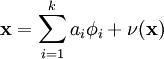
Consider the problem of modelling natural images as the linear superposition of $k$ independent source features $\mathbf{\phi}_i$ with some additive noise $ν$ :

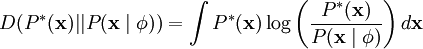
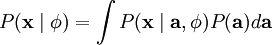
$\begin{align}\mathbf{x} = \sum_{i=1}^k a_i \mathbf{\phi}_{i} + \nu(\mathbf{x})\end{align}$

Our goal is to find a set of basis feature vectors $\mathbf{\phi}$ such that the distribution of images $P(\mathbf{x}\mid\mathbf{\phi})$ is as close as possible to the empirical distribution of our input data $P^*(\mathbf{x})$ . One method of doing so is to minimize the KL divergence between $P^*(\mathbf{x})$ and $P(\mathbf{x}\mid\mathbf{\phi})$ where the KL divergence is defined as:

$\begin{align}D(P^*(\mathbf{x})||P(\mathbf{x}\mid\mathbf{\phi})) = \int P^*(\mathbf{x}) \log \left(\frac{P^*(\mathbf{x})}{P(\mathbf{x}\mid\mathbf{\phi})}\right)d\mathbf{x}\end{align}$

Since the empirical distribution $P^*(\mathbf{x})$ is constant across our choice of $\mathbf{\phi}$ , this is equivalent to maximizing the log-likelihood of $P(\mathbf{x}\mid\mathbf{\phi})$ .

Assuming $ν$ is Gaussian white noise with variance $σ 2$ , we have that

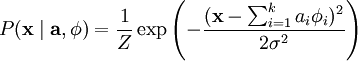
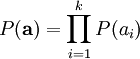
$\begin{align}P(\mathbf{x} \mid \mathbf{a}, \mathbf{\phi}) = \frac{1}{Z} \exp\left(- \frac{(\mathbf{x}-\sum^{k}_{i=1} a_i \mathbf{\phi}_{i})^2}{2\sigma^2}\right)\end{align}$

In order to determine the distribution $P(\mathbf{x}\mid\mathbf{\phi})$ , we also need to specify the prior distribution $P(\mathbf{a})$ . Assuming the independence of our source features, we can factorize our prior probability as

$\begin{align}P(\mathbf{a}) = \prod_{i=1}^{k} P(a_i)\end{align}$

At this point, we would like to incorporate our sparsity assumption -- the assumption that any single image is likely to be the product of relatively few source features. Therefore, we would like the probability distribution of $a i$ to be peaked at zero and have high kurtosis. A convenient parameterization of the prior distribution is

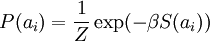
$\begin{align}P(a_i) = \frac{1}{Z}\exp(-\beta S(a_i))\end{align}$

Where $S (a i)$ is a function determining the shape of the prior distribution.

Having defined $P(\mathbf{x} \mid \mathbf{a}, \mathbf{\phi})$ and $P(\mathbf{a})$ , we can write the probability of the data $\mathbf{x}$ under the model defined by $\mathbf{\phi}$ as

$\begin{align}P(\mathbf{x} \mid \mathbf{\phi}) = \int P(\mathbf{x} \mid \mathbf{a}, \mathbf{\phi}) P(\mathbf{a}) d\mathbf{a}\end{align}$

and our problem reduces to finding

$\begin{align}\mathbf{\phi}^*=\text{argmax}_{\mathbf{\phi}} < \log(P(\mathbf{x} \mid \mathbf{\phi})) >\end{align}$

Where $< . >$ denotes expectation over our input data.

Unfortunately, the integral over $\mathbf{a}$ to obtain $P(\mathbf{x} \mid \mathbf{\phi})$ is generally intractable. We note though that if the distribution of $P(\mathbf{x} \mid \mathbf{\phi})$ is sufficiently peaked (w.r.t. $\mathbf{a}$ ), we can approximate its integral with the maximum value of $P(\mathbf{x} \mid \mathbf{\phi})$ and obtain a approximate solution

$\begin{align}\mathbf{\phi}^{*'}=\text{argmax}_{\mathbf{\phi}} < \max_{\mathbf{a}} \log(P(\mathbf{x} \mid \mathbf{\phi})) >\end{align}$

As before, we may increase the estimated probability by scaling down $a i$ and scaling up $\mathbf{\phi}$ (since $P (a i)$ peaks about zero) , we therefore impose a norm constraint on our features $\mathbf{\phi}$ to prevent this.

Finally, we can recover our original cost function by defining the energy function of this linear generative model

$\begin{array}{rl}E\left( \mathbf{x} , \mathbf{a} \mid \mathbf{\phi} \right) & := -\log \left( P(\mathbf{x}\mid \mathbf{\phi},\mathbf{a}\right)P(\mathbf{a})) \\ &= \sum_{j=1}^{m} \left|\left| \mathbf{x}^{(j)} - \sum_{i=1}^k a^{(j)}_i \mathbf{\phi}_{i}\right|\right|^{2} + \lambda \sum_{i=1}^{k}S(a^{(j)}_i) \end{array}$

where $λ = 2σ 2 β$ and irrelevant constants have been hidden. Since maximizing the log-likelihood is equivalent to minimizing the energy function, we recover the original optimization problem:

$\begin{align}\mathbf{\phi}^{*},\mathbf{a}^{*}=\text{argmin}_{\mathbf{\phi},\mathbf{a}} \sum_{j=1}^{m} \left|\left| \mathbf{x}^{(j)} - \sum_{i=1}^k a^{(j)}_i \mathbf{\phi}_{i}\right|\right|^{2} + \lambda \sum_{i=1}^{k}S(a^{(j)}_i) \end{align}$

Using a probabilistic approach, it can also be seen that the choices of the $L 1$ penalty $\left|a_i\right|_1$ and the log penalty $\log(1+a_i^2)$ for $S (.)$ correspond to the use of the Laplacian 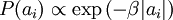$P(a_i) \propto \exp\left(-\beta|a_i|\right)$ and the Cauchy prior 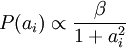$P(a_i) \propto \frac{\beta}{1+a_i^2}$ respectively.

Learning

Learning a set of basis vectors $\mathbf{\phi}$ using sparse coding consists of performing two separate optimizations, the first being an optimization over coefficients $a i$ for each training example $\mathbf{x}$ and the second an optimization over basis vectors $\mathbf{\phi}$ across many training examples at once.

Assuming an $L 1$ sparsity penalty, learning $a^{(j)}_i$ reduces to solving a $L 1$ regularized least squares problem which is convex in $a^{(j)}_i$ for which several techniques have been developed (convex optimization software such as CVX can also be used to perform L1 regularized least squares). Assuming a differentiable $S (.)$ such as the log penalty, gradient-based methods such as conjugate gradient methods can also be used.

Learning a set of basis vectors with a $L 2$ norm constraint also reduces to a least squares problem with quadratic constraints which is convex in $\mathbf{\phi}$ . Standard convex optimization software (e.g. CVX) or other iterative methods can be used to solve for $\mathbf{\phi}$ although significantly more efficient methods such as solving the Lagrange dual have also been developed.

As described above, a significant limitation of sparse coding is that even after a set of basis vectors have been learnt, in order to "encode" a new data example, optimization must be performed to obtain the required coefficients. This significant "runtime" cost means that sparse coding is computationally expensive to implement even at test time especially compared to typical feedforward architectures.

Sparse Coding: Autoencoder Interpretation

[hide]

1 Sparse coding
2 Topographic sparse coding
3 Sparse coding in practice
- 3.1 Batching examples into mini-batches
- 3.2 Good initialization of s
- 3.3 The practical algorithm

Sparse coding

In the sparse autoencoder, we tried to learn a set of weights $W$ (and associated biases $b$ ) that would give us sparse features $σ(Wx + b)$ useful in reconstructing the input $x$ .

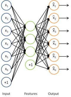
Sparse coding can be seen as a modification of the sparse autoencoder method in which we try to learn the set of features for some data "directly". Together with an associated basis for transforming the learned features from the feature space to the data space, we can then reconstruct the data from the learned features.

Formally, in sparse coding, we have some data $x$ we would like to learn features on. In particular, we would like to learn $s$ , a set of sparse features useful for representing the data, and $A$ , a basis for transforming the features from the feature space to the data space. Our objective function is hence:

$J(A, s) = \lVert As - x \rVert_2^2 + \lambda \lVert s \rVert_1$

(If you are unfamiliar with the notation, $\lVert x \rVert_k$ refers to the L $k$ norm of the $x$ which is equal to $\left( \sum{ \left| x_i^k \right| } \right) ^{\frac{1}{k}}$ . The L2 norm is the familiar Euclidean norm, while the L1 norm is the sum of absolute values of the elements of the vector)

The first term is the error in reconstructing the data from the features using the basis, and the second term is a sparsity penalty term to encourage the learned features to be sparse.

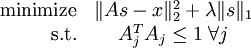
However, the objective function as it stands is not properly constrained - it is possible to reduce the sparsity cost (the second term) by scaling $A$ by some constant and scaling $s$ by the inverse of the same constant, without changing the error. Hence, we include the additional constraint that that for every column $A j$ of $A$ , $A_j^TA_j \le 1$ . Our problem is thus:

$\begin{array}{rcl} {\rm minimize} & \lVert As - x \rVert_2^2 + \lambda \lVert s \rVert_1 \\ {\rm s.t.} & A_j^TA_j \le 1 \; \forall j \\\end{array}$

Unfortunately, the objective function is non-convex, and hence impossible to optimize well using gradient-based methods. However, given $A$ , the problem of finding $s$ that minimizes $J (A, s)$ is convex. Similarly, given $s$ , the problem of finding $A$ that minimizes $J (A, s)$ is also convex. This suggests that we might try alternately optimizing for $A$ for a fixed $s$ , and then optimizing for $s$ given a fixed $A$ . It turns out that this works quite well in practice.

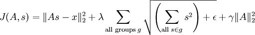
However, the form of our problem presents another difficulty - the constraint that $A_j^TA_j \le 1 \; \forall j$ cannot be enforced using simple gradient-based methods. Hence, in practice, this constraint is weakened to a "weight decay" term designed to keep the entries of $A$ small. This gives us a new objective function:

$J(A, s) = \lVert As - x \rVert_2^2 + \lambda \lVert s \rVert_1 + \gamma \lVert A \rVert_2^2$

(note that the third term, $\lVert A \rVert_2^2$ is simply the sum of squares of the entries of A, or $\sum_r{\sum_c{A_{rc}^2}}$ )

This objective function presents one last problem - the L1 norm is not differentiable at 0, and hence poses a problem for gradient-based methods. While the problem can be solved using other non-gradient descent-based methods, we will "smooth out" the L1 norm using an approximation which will allow us to use gradient descent. To "smooth out" the L1 norm, we use $\sqrt{x^2 + \epsilon}$ in place of $\left| x \right|$ , where $ε$ is a "smoothing parameter" which can also be interpreted as a sort of "sparsity parameter" (to see this, observe that when $ε$ is large compared to $x$ , the $x + ε$ is dominated by $ε$ , and taking the square root yields approximately $\sqrt{\epsilon}$ ). This "smoothing" will come in handy later when considering topographic sparse coding below.

Our final objective function is hence:

$J(A, s) = \lVert As - x \rVert_2^2 + \lambda \sqrt{s^2 + \epsilon} + \gamma \lVert A \rVert_2^2$

(where $\sqrt{s^2 + \epsilon}$ is shorthand for $\sum_k{\sqrt{s_k^2 + \epsilon}}$ )

This objective function can then be optimized iteratively, using the following procedure:

Initialize $A$ randomly
Repeat until convergence
1. Find the $s$ that minimizes $J (A, s)$ for the $A$ found in the previous step
2. Solve for the $A$ that minimizes $J (A, s)$ for the $s$ found in the previous step

Observe that with our modified objective function, the objective function $J (A, s)$ given $s$ , that is $J(A; s) = \lVert As - x \rVert_2^2 + \gamma \lVert A \rVert_2^2$ (the L1 term in $s$ can be omitted since it is not a function of $A$ ) is simply a quadratic term in $A$ , and hence has an easily derivable analytic solution in $A$ . A quick way to derive this solution would be to use matrix calculus - some pages about matrix calculus can be found in the useful links section. Unfortunately, the objective function given $A$ does not have a similarly nice analytic solution, so that minimization step will have to be carried out using gradient descent or similar optimization methods.

In theory, optimizing for this objective function using the iterative method as above should (eventually) yield features (the basis vectors of $A$ ) similar to those learned using the sparse autoencoder. However, in practice, there are quite a few tricks required for better convergence of the algorithm, and these tricks are described in greater detail in the later section on sparse coding in practice. Deriving the gradients for the objective function may be slightly tricky as well, and using matrix calculus or using the backpropagation intuition can be helpful.

Topographic sparse coding

With sparse coding, we can learn a set of features useful for representing the data. However, drawing inspiration from the brain, we would like to learn a set of features that are "orderly" in some manner. For instance, consider visual features. As suggested earlier, the V1 cortex of the brain contains neurons which detect edges at particular orientations. However, these neurons are also organized into hypercolumns in which adjacent neurons detect edges at similar orientations. One neuron could detect a horizontal edge, its neighbors edges oriented slightly off the horizontal, and moving further along the hypercolumn, the neurons detect edges oriented further off the horizontal.

Inspired by this example, we would like to learn features which are similarly "topographically ordered". What does this imply for our learned features? Intuitively, if "adjacent" features are "similar", we would expect that if one feature is activated, its neighbors will also be activated to a lesser extent.

Concretely, suppose we (arbitrarily) organized our features into a square matrix. We would then like adjacent features in the matrix to be similar. The way this is accomplished is to group these adjacent features together in the smoothed L1 penalty, so that instead of say $\sqrt{s_{1,1}^2 + \epsilon}$ , we use say $\sqrt{s_{1,1}^2 + s_{1,2}^2 + s_{1,3}^2 + s_{2,1}^2 + s_{2,2}^2 + s_{3,2}^2 + s_{3,1}^2 + s_{3,2}^2 + s_{3,3}^2 + \epsilon}$ instead, if we group in 3x3 regions. The grouping is usually overlapping, so that the 3x3 region starting at the 1st row and 1st column is one group, the 3x3 region starting at the 1st row and 2nd column is another group, and so on. Further, the grouping is also usually done wrapping around, as if the matrix were a torus, so that every feature is counted an equal number of times.

Hence, in place of the smoothed L1 penalty, we use the sum of smoothed L1 penalties over all the groups, so our new objective function is:

$J(A, s) = \lVert As - x \rVert_2^2 + \lambda \sum_{\text{all groups } g}{\sqrt{ \left( \sum_{\text{all } s \in g}{s^2} \right) + \epsilon} } + \gamma \lVert A \rVert_2^2$

In practice, the "grouping" can be accomplished using a "grouping matrix" $V$ , such that the $r$ th row of $V$ indicates which features are grouped in the $r$ th group, so $V r, c = 1$ if group $r$ contains feature $c$ . Thinking of the grouping as being achieved by a grouping matrix makes the computation of the gradients more intuitive. Using this grouping matrix, the objective function can be rewritten as:

$J(A, s) = \lVert As - x \rVert_2^2 + \lambda \sum{ \sqrt{Vss^T + \epsilon} } + \gamma \lVert A \rVert_2^2$

(where $\sum{ \sqrt{Vss^T + \epsilon} }$ is

∑∑D_r,crc

if we let $D = \sqrt{Vss^T + \epsilon}$ )

This objective function can be optimized using the iterated method described in the earlier section. Topographic sparse coding will learn features similar to those learned by sparse coding, except that the features will now be "ordered" in some way.

Sparse coding in practice

As suggested in the earlier sections, while the theory behind sparse coding is quite simple, writing a good implementation that actually works and converges reasonably quickly to good optima requires a bit of finesse.

Recall the simple iterative algorithm proposed earlier:

Initialize $A$ randomly
Repeat until convergence
1. Find the $s$ that minimizes $J (A, s)$ for the $A$ found in the previous step
2. Solve for the $A$ that minimizes $J (A, s)$ for the $s$ found in the previous step

It turns out that running this algorithm out of the box will not produce very good results, if any results are produced at all. There are two main tricks to achieve faster and better convergence:

Batching examples into "mini-batches"
Good initialization of $s$

Batching examples into mini-batches

If you try running the simple iterative algorithm on a large dataset of say 10 000 patches at one go, you will find that each iteration takes a long time, and the algorithm may hence take a long time to converge. To increase the rate of convergence, you can instead run the algorithm on mini-batches instead. To do this, instead of running the algorithm on all 10 000 patches, in each iteration, select a mini-batch - a (different) random subset of say 2000 patches from the 10 000 patches - and run the algorithm on that mini-batch for the iteration instead. This accomplishes two things - firstly, it speeds up each iteration, since now each iteration is operating on 2000 rather than 10 000 patches; secondly, and more importantly, it increases the rate of convergence(TODO: explain why).

Good initialization of $s$

Another important trick in obtaining faster and better convergence is good initialization of the feature matrix $s$ before using gradient descent (or other methods) to optimize for the objective function for $s$ given $A$ . In practice, initializing $s$ randomly at each iteration can result in poor convergence unless a good optima is found for $s$ before moving on to optimize for $A$ . A better way to initialize $s$ is the following:

Set $s \leftarrow W^Tx$ (where $x$ is the matrix of patches in the mini-batch)
For each feature in $s$ (i.e. each column of $s$ ), divide the feature by the norm of the corresponding basis vector in $A$ . That is, if $s r, c$ is the $r$ th feature for the $c$ th example, and $A c$ is the $c$ th basis vector in $A$ , then set $s_{r, c} \leftarrow \frac{ s_{r, c} } { \lVert A_c \rVert }.$

Very roughly and informally speaking, this initialization helps because the first step is an attempt to find a good $s$ such that $Ws \approx x$ , and the second step "normalizes" $s$ in an attempt to keep the sparsity penalty small. It turns out that initializing $s$ using only one but not both steps results in poor performance in practice. (TODO: a better explanation for why this initialization helps?)

The practical algorithm

With the above two tricks, the algorithm for sparse coding then becomes:

Initialize $A$ randomly
Repeat until convergence
1. Select a random mini-batch of 2000 patches
2. Initialize $s$ as described above
3. Find the $s$ that minimizes $J (A, s)$ for the $A$ found in the previous step
4. Solve for the $A$ that minimizes $J (A, s)$ for the $s$ found in the previous step

With this method, you should be able to reach a good local optima relatively quickly.

Exercise:Sparse Coding

[hide]

1 Sparse Coding
- 1.1 Dependencies
- 1.2 Step 0: Initialization
- 1.3 Step 1: Sample patches
- 1.4 Step 2: Implement and check sparse coding cost functions
- 1.5 Step 3: Iterative optimization

Sparse Coding

In this exercise, you will implement sparse coding and topographic sparse coding on black-and-white natural images.

In the file sparse_coding_exercise.zip we have provided some starter code. You should write your code at the places indicated "YOUR CODE HERE" in the files.

For this exercise, you will need to modify sparseCodingWeightCost.m, sparseCodingFeatureCost.m and sparseCodingExercise.m.

Dependencies

You will need:

computeNumericalGradient.m from Exercise:Sparse Autoencoder
display_network.m from Exercise:Sparse Autoencoder

If you have not completed the exercise listed above, we strongly suggest you complete it first.

Step 0: Initialization

In this step, we initialize some parameters used for the exercise.

Step 1: Sample patches

In this step, we sample some patches from the IMAGES.mat dataset comprising 10 black-and-white pre-whitened natural images.

Step 2: Implement and check sparse coding cost functions

In this step, you should implement the two sparse coding cost functions:

sparseCodingWeightCost in sparseCodingWeightCost.m, which is used for optimizing the weight cost given the features
sparseCodingFeatureCost in sparseCodingFeatureCost.m, which is used for optimizing the feature cost given the weights

Each of these functions should compute the appropriate cost and gradient. You may wish to implement the non-topographic version ofsparseCodingFeatureCost first, ignoring the grouping matrix and assuming that none of the features are grouped. You can then extend this to the topographic version later. Alternatively, you may implement the topographic version directly - using the non-topographic version will then involve setting the grouping matrix to the identity matrix.

Once you have implemented these functions, you should check the gradients numerically.

Implementation tip - gradient checking the feature cost. One particular point to note is that when checking the gradient for the feature cost, epsilon should be set to a larger value, for instance 1e-2 (as has been done for you in the checking code provided), to ensure that checking the gradient numerically makes sense. This is necessary because as epsilon becomes smaller, the function sqrt(x + epsilon) becomes "sharper" and more "pointed", making the numerical gradient computed near 0 less and less accurate. To see this, consider what would happen if the numerical gradient was computed by using a point with x less than 0 and a point with x greater than 0 - the computed numerical slope would be wildly inaccurate.

Step 3: Iterative optimization

In this step, you will iteratively optimize for the weights and features to learn a basis for the data, as described in the section on sparse coding. Mini-batching and initialization of the features $s$ has already been done for you. However, you need to still need to fill in the analytic solution to the the optimization problem with respect to the weight matrix, given the feature matrix.

Once that is done, you should check that your solution is correct using the given checking code, which checks that the gradient at the point determined by your analytic solution is close to 0. Once your solution has been verified, comment out the checking code, and run the iterative optimization code. 200 iterations should take less than 45 minutes to run, and by 100 iterations you should be able to see bases that look like edges, similar to those you learned in the sparse autoencoder exercise.

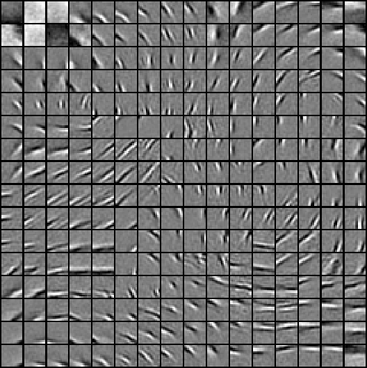
For the non-topographic case, these features will not be "ordered", and will look something like the following:

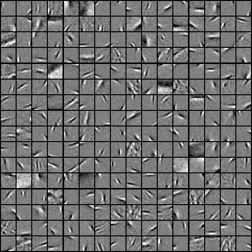
For the topographic case, the features will be "ordered topographically", and will look something like the following:

CS294A/CS294W Sparse Coding Exercise
STEP 0: Initialization
STEP 1: Sample patches
STEP 3: Iterative optimization

CS294A/CS294W Sparse Coding Exercise

%  Instructions%  ------------%%  This file contains code that helps you get started on the%  sparse coding exercise. In this exercise, you will need to modify%  sparseCodingFeatureCost.m and sparseCodingWeightCost.m. You will also%  need to modify this file, sparseCodingExercise.m slightly.% Add the paths to your earlier exercises if necessary% addpath /path/to/solution%%======================================================================

STEP 0: Initialization

Here we initialize some parameters used for the exercise.

addpath minFunc;numPatches = 1000;   % number of patchesnumFeatures = 121;    % number of features to learnpatchDim = 8;         % patch dimensionvisibleSize = patchDim * patchDim; %单通道灰度图，64维，学习121个特征% dimension of the grouping region (poolDim x poolDim) for topographic sparse codingpoolDim = 3;% number of patches per batchbatchNumPatches = 200; %分成5个batchlambda = 5e-5;  % L1-regularisation parameter (on features)epsilon = 1e-5; % L1-regularisation epsilon |x| ~ sqrt(x^2 + epsilon)gamma = 1e-2;   % L2-regularisation parameter (on basis)%%======================================================================

STEP 1: Sample patches

images = load('IMAGES.mat');images = images.IMAGES;patches = sampleIMAGES(images, patchDim, numPatches);display_network(patches(:, 1:64));%%======================================================================

STEP 3: Iterative optimization

Once you have implemented the cost functions, you can now optimize forthe objective iteratively. The code to do the iterative optimizationusing mini-batching and good initialization of the features has alreadybeen included for you.

However, you will still need to derive and fill in the analytic solutionfor optimizing the weight matrix given the features.Derive the solution and implement it in the code below, verify thegradient as described in the instructions below, and then run theiterative optimization.

% Initialize options for minFuncoptions.Method = 'cg';options.display = 'on';options.verbose = 0;% Initialize matricesweightMatrix = rand(visibleSize, numFeatures);%64*121featureMatrix = rand(numFeatures, batchNumPatches);%121*2000% Initialize grouping matrixassert(floor(sqrt(numFeatures)) ^2 == numFeatures, 'numFeatures should be a perfect square');donutDim = floor(sqrt(numFeatures));assert(donutDim * donutDim == numFeatures,'donutDim^2 must be equal to numFeatures');groupMatrix = zeros(numFeatures, donutDim, donutDim);%121*11*11groupNum = 1;for row = 1:donutDim    for col = 1:donutDim        groupMatrix(groupNum, 1:poolDim, 1:poolDim) = 1;%poolDim=3        groupNum = groupNum + 1;        groupMatrix = circshift(groupMatrix, [0 0 -1]);    end    groupMatrix = circshift(groupMatrix, [0 -1, 0]);endgroupMatrix = reshape(groupMatrix, numFeatures, numFeatures);%121*121if isequal(questdlg('Initialize grouping matrix for topographic or non-topographic sparse coding?', 'Topographic/non-topographic?', 'Non-topographic', 'Topographic', 'Non-topographic'), 'Non-topographic')    groupMatrix = eye(numFeatures);%非拓扑结构时的groupMatrix矩阵end% Initial batchindices = randperm(numPatches);%1*20000indices = indices(1:batchNumPatches);%1*2000batchPatches = patches(:, indices);fprintf('%6s%12s%12s%12s%12s\n','Iter', 'fObj','fResidue','fSparsity','fWeight');warning off;for iteration = 1:200  %  iteration = 1;    error = weightMatrix * featureMatrix - batchPatches;    error = sum(error(:) .^ 2) / batchNumPatches;  %说明重构误差需要考虑样本数    fResidue = error;    num_batches = size(batchPatches,2);    R = groupMatrix * (featureMatrix .^ 2);    R = sqrt(R + epsilon);    fSparsity = lambda * sum(R(:));    %稀疏项和权值惩罚项不需要考虑样本数    fWeight = gamma * sum(weightMatrix(:) .^ 2);    %上面的那些权值都是随机初始化的    fprintf('  %4d  %10.4f  %10.4f  %10.4f  %10.4f\n', iteration, fResidue+fSparsity+fWeight, fResidue, fSparsity, fWeight)    % Select a new batch    indices = randperm(numPatches);    indices = indices(1:batchNumPatches);    batchPatches = patches(:, indices);    % Reinitialize featureMatrix with respect to the new    % 对featureMatrix重新初始化，按照网页教程上介绍的方法进行    featureMatrix = weightMatrix' * batchPatches;    normWM = sum(weightMatrix .^ 2)';    featureMatrix = bsxfun(@rdivide, featureMatrix, normWM);    % Optimize for feature matrix    options.maxIter = 20;    %给定权值初始值，优化特征值矩阵    [featureMatrix, cost] = minFunc( @(x) sparseCodingFeatureCost(weightMatrix, x, visibleSize, numFeatures, batchPatches, gamma, lambda, epsilon, groupMatrix), ...                                           featureMatrix(:), options);    featureMatrix = reshape(featureMatrix, numFeatures, batchNumPatches);    %jie xi jie    weightMatrix = (batchPatches*featureMatrix')/(gamma*num_batches*eye(size(featureMatrix,1))+featureMatrix*featureMatrix');    [cost, grad] = sparseCodingWeightCost(weightMatrix, featureMatrix, visibleSize, numFeatures, batchPatches, gamma, lambda, epsilon, groupMatrix);end    totalElem=size(featureMatrix,1)*size(featureMatrix,2);    ave=sum(featureMatrix(:))/totalElem    ind=find(abs(featureMatrix)<0.001);    sparseRate=numel(ind)/totalElem    ind=find(abs(featureMatrix)<0.001);    featureMatrix2=featureMatrix;    featureMatrix2(ind)=0;    aaaa=featureMatrix2(1,:);    save('save/my.mat','featureMatrix','weightMatrix')    figure;    display_network(weightMatrix);

Contents
求目标的代价函数
求目标代价函数的偏导函数
function [cost, grad] = sparseCodingFeatureCost(weightMatrix, featureMatrix, visibleSize, numFeatures, patches, gamma, lambda, epsilon, groupMatrix)
%sparseCodingFeatureCost - given the weights in weightMatrix,%                          computes the cost and gradient with respect to%                          the features, given in featureMatrix% parameters%   weightMatrix  - the weight matrix. weightMatrix(:, c) is the cth basis%                   vector.%   featureMatrix - the feature matrix. featureMatrix(:, c) is the features%                   for the cth example%   visibleSize   - number of pixels in the patches%   numFeatures   - number of features%   patches       - patches%   gamma         - weight decay parameter (on weightMatrix)%   lambda        - L1 sparsity weight (on featureMatrix)%   epsilon       - L1 sparsity epsilon%   groupMatrix   - the grouping matrix. groupMatrix(r, :) indicates the%                   features included in the rth group. groupMatrix(r, c)%                   is 1 if the cth feature is in the rth group and 0%                   otherwise.    isTopo = 1;%     L = size(groupMatrix,1);%     [K M] = size(featureMatrix);    if exist('groupMatrix', 'var')        assert(size(groupMatrix, 2) == numFeatures, 'groupMatrix has bad dimension');        if(isequal(groupMatrix,eye(numFeatures)));            isTopo = 0;        end    else        groupMatrix = eye(numFeatures);         isTopo = 0;    end    numExamples = size(patches, 2);    weightMatrix = reshape(weightMatrix, visibleSize, numFeatures);    featureMatrix = reshape(featureMatrix, numFeatures, numExamples);    % -------------------- YOUR CODE HERE --------------------    % Instructions:    %   Write code to compute the cost and gradient with respect to the    %   features given in featureMatrix.    %   You may wish to write the non-topographic version, ignoring    %   the grouping matrix groupMatrix first, and extend the    %   non-topographic version to the topographic version later.    % -------------------- YOUR CODE HERE --------------------
求目标的代价函数
    delta = weightMatrix*featureMatrix-patches;    fResidue = sum(sum(delta.^2))./numExamples;%重构误差%     fWeight = gamma*sum(sum(weightMatrix.^2));%防止基内元素值过大    sparsityMatrix = sqrt(groupMatrix*(featureMatrix.^2)+epsilon);    fSparsity = lambda*sum(sparsityMatrix(:)); %对特征系数性的惩罚值%     cost = fResidue++fSparsity+fWeight;%此时A为常量，可以不用    cost = fResidue++fSparsity;
求目标代价函数的偏导函数
    gradResidue = (-2*weightMatrix'*patches+2*weightMatrix'*weightMatrix*featureMatrix)./numExamples;    % 非拓扑结构时：    if ~isTopo        gradSparsity = lambda*(featureMatrix./sparsityMatrix);    end    % 拓扑结构时    if isTopo%         gradSparsity = lambda*groupMatrix'*(groupMatrix*(featureMatrix.^2)+epsilon).^(-0.5).*featureMatrix;%一定要小心最后一项是内积乘法        gradSparsity = lambda*groupMatrix'*(groupMatrix*(featureMatrix.^2)+epsilon).^(-0.5).*featureMatrix;%一定要小心最后一项是内积乘法    end    grad = gradResidue+gradSparsity;    grad = grad(:);
end

Contents
求目标的代价函数
求目标代价函数的偏导函数
function [cost, grad] = sparseCodingWeightCost(weightMatrix, featureMatrix, visibleSize, numFeatures,  patches, gamma, lambda, epsilon, groupMatrix)
%sparseCodingWeightCost - given the features in featureMatrix,%                         computes the cost and gradient with respect to%                         the weights, given in weightMatrix% parameters%   weightMatrix  - the weight matrix. weightMatrix(:, c) is the cth basis%                   vector.%   featureMatrix - the feature matrix. featureMatrix(:, c) is the features%                   for the cth example%   visibleSize   - number of pixels in the patches%   numFeatures   - number of features%   patches       - patches%   gamma         - weight decay parameter (on weightMatrix)%   lambda        - L1 sparsity weight (on featureMatrix)%   epsilon       - L1 sparsity epsilon%   groupMatrix   - the grouping matrix. groupMatrix(r, :) indicates the%                   features included in the rth group. groupMatrix(r, c)%                   is 1 if the cth feature is in the rth group and 0%                   otherwise.    if exist('groupMatrix', 'var')        assert(size(groupMatrix, 2) == numFeatures, 'groupMatrix has bad dimension');    else        groupMatrix = eye(numFeatures);%非拓扑的sparse coding中，相当于groupMatrix为单位对角矩阵    end    numExamples = size(patches, 2);%测试代码时为5    weightMatrix = reshape(weightMatrix, visibleSize, numFeatures);%其实传入进来的就是这些东西    featureMatrix = reshape(featureMatrix, numFeatures, numExamples);    % -------------------- YOUR CODE HERE --------------------    % Instructions:    %   Write code to compute the cost and gradient with respect to the    %   weights given in weightMatrix.    % -------------------- YOUR CODE HERE --------------------
Input argument "numFeatures" is undefined.Error in ==> sparseCodingWeightCost at 24        groupMatrix = eye(numFeatures);%非拓扑的sparse coding中，相当于groupMatrix为单位对角矩阵
求目标的代价函数
    delta = weightMatrix*featureMatrix-patches;    fResidue = sum(sum(delta.^2))./numExamples;%重构误差    fWeight = gamma*sum(sum(weightMatrix.^2));%防止基内元素值过大%     sparsityMatrix = sqrt(groupMatrix*(featureMatrix.^2)+epsilon);%     fSparsity = lambda*sum(sparsityMatrix(:)); %对特征系数性的惩罚值%     cost = fResidue+fWeight+fSparsity; %目标的代价函数    cost = fResidue+fWeight;
求目标代价函数的偏导函数
    grad = (2*weightMatrix*featureMatrix*featureMatrix'-2*patches*featureMatrix')./numExamples+2*gamma*weightMatrix;    grad = grad(:);
end

0 0

UFLDL Tutorial_Sparse Coding

Sparse Coding

Sparse Coding

Probabilistic Interpretation [Based on Olshausen and Field 1996]

Learning

Sparse Coding: Autoencoder Interpretation

Contents

Sparse coding

Topographic sparse coding

Sparse coding in practice

Batching examples into mini-batches

Good initialization of s

The practical algorithm

Exercise:Sparse Coding

Contents

Sparse Coding

Dependencies

Step 0: Initialization

Step 1: Sample patches

Step 2: Implement and check sparse coding cost functions

Step 3: Iterative optimization

Contents

CS294A/CS294W Sparse Coding Exercise

STEP 0: Initialization

STEP 1: Sample patches

STEP 3: Iterative optimization

Contents

求目标的代价函数

求目标代价函数的偏导函数

Contents

求目标的代价函数

求目标代价函数的偏导函数

Good initialization of $s$