UFLDL Tutorial_ICA Style Models

Independent Component Analysis

Introduction

If you recall, in sparse coding, we wanted to learn an over-complete basis for the data. In particular, this implies that the basis vectors that we learn in sparse coding will not be linearly independent. While this may be desirable in certain situations, sometimes we want to learn a linearly independent basis for the data. In independent component analysis (ICA), this is exactly what we want to do. Further, in ICA, we want to learn not just any linearly independent basis, but an orthonormal basis for the data. (An orthonormal basis is a basis  such that  if  and 1 if i = j).

Like sparse coding, independent component analysis has a simple mathematical formulation. Given some data x, we would like to learn a set of basis vectors which we represent in the columns of a matrix W, such that, firstly, as in sparse coding, our features aresparse; and secondly, our basis is an orthonormal basis. (Note that while in sparse coding, our matrix A was for mappingfeatures s to raw data, in independent component analysis, our matrix W works in the opposite direction, mapping raw data x tofeatures instead). This gives us the following objective function:

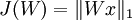
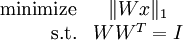
This objective function is equivalent to the sparsity penalty on the features s in sparse coding, since Wx is precisely the features that represent the data. Adding in the orthonormality constraint gives us the full optimization problem for independent component analysis:

As is usually the case in deep learning, this problem has no simple analytic solution, and to make matters worse, the orthonormality constraint makes it slightly more difficult to optimize for the objective using gradient descent - every iteration of gradient descent must be followed by a step that maps the new basis back to the space of orthonormal bases (hence enforcing the constraint).

In practice, optimizing for the objective function while enforcing the orthonormality constraint (as described in Orthonormal ICAsection below) is feasible but slow. Hence, the use of orthonormal ICA is limited to situations where it is important to obtain an orthonormal basis (TODO: what situations) .

Orthonormal ICA

The orthonormal ICA objective is:

Observe that the constraint WW^T = I implies two other constraints.

Firstly, since we are learning an orthonormal basis, the number of basis vectors we learn must be less than the dimension of the input. In particular, this means that we cannot learn over-complete bases as we usually do in sparse coding.

Secondly, the data must be ZCA whitened with no regularization (that is, with ε set to 0). (TODO Why must this be so?)

Hence, before we even begin to optimize for the orthonormal ICA objective, we must ensure that our data has been whitened, and that we are learning an under-complete basis.

Following that, to optimize for the objective, we can use gradient descent, interspersing gradient descent steps with projection steps to enforce the orthonormality constraint. Hence, the procedure will be as follows:

Repeat until done:

1. 
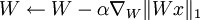
2.  where U is the space of matrices satisfying WW^T = I

In practice, the learning rate α is varied using a line-search algorithm to speed up the descent, and the projection step is achieved by setting , which can actually be seen as ZCA whitening (TODO explain how it is like ZCA whitening).

Topographic ICA

Just like sparse coding, independent component analysis can be modified to give a topographic variant by adding a topographic cost term.

Exercise:Independent Component Analysis

Contents

 [hide]

• 1 Independent Component Analysis
  • 1.1 Dependencies
  • 1.2 Step 0: Initialization
  • 1.3 Step 1: Sample patches
  • 1.4 Step 2: ZCA whiten patches
  • 1.5 Step 3: Implement and check ICA cost functions
    • 1.5.1 Step 4: Optimization
  • 1.6 Appendix
    • 1.6.1 Backtracking line search

Independent Component Analysis

In this exercise, you will implement Independent Component Analysis on color images from the STL-10 dataset.

In the file independent_component_analysis_exercise.zip we have provided some starter code. You should write your code at the places indicated "YOUR CODE HERE" in the files.

For this exercise, you will need to modify OrthonormalICACost.m and ICAExercise.m.

Dependencies

You will need:

• computeNumericalGradient.m from Exercise:Sparse Autoencoder
• displayColorNetwork.m from Exercise:Learning color features with Sparse Autoencoders

The following additional file is also required for this exercise:

• Sampled 8x8 patches from the STL-10 dataset (stl10_patches_100k.zip)

If you have not completed the exercises listed above, we strongly suggest you complete them first.

Step 0: Initialization

In this step, we initialize some parameters used for the exercise.

Step 1: Sample patches

In this step, we load and use a portion of the 8x8 patches from the STL-10 dataset (which you first saw in the exercise on linear decoders).

Step 2: ZCA whiten patches

In this step, we ZCA whiten the patches as required by orthonormal ICA.

Step 3: Implement and check ICA cost functions

In this step, you should implement the ICA cost function: orthonormalICACost in orthonormalICACost.m, which computes the cost and gradient for the orthonormal ICA objective. Note that the orthonormality constraint is not enforced in the cost function. It will be enforced by a projection in the gradient descent step, which you will have to complete in step 4.

When you have implemented the cost function, you should check the gradients numerically.

Hint - if you are having difficulties deriving the gradients, you may wish to consult the page on deriving gradients using the backpropagation idea.

Step 4: Optimization

In step 4, you will optimize for the orthonormal ICA objective using gradient descent with backtracking line search (the code for which has already been provided for you. For more details on the backtracking line search, you may wish to consult the appendix of this exercise). The orthonormality constraint should be enforced with a projection, which you should fill in.

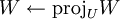
Once you have filled in the code for the projection, check that it is correct by using the verification code provided. Once you have verified that your projection is correct, comment out the verification code and run the optimization. 1000 iterations of gradient descent should take less than 15 minutes, and produce a basis which looks like the following:

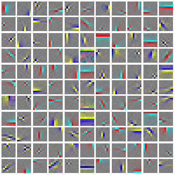
It is comparatively difficult to optimize for the objective while enforcing the orthonormality constraint using gradient descent, and convergence can be slow. Hence, in situations where an orthonormal basis is not required, other faster methods of learning bases (such as sparse coding) may be preferable.

Appendix

Backtracking line search

The backtracking line search used in the exercise is based off that in Convex Optimization by Boyd and Vandenbergh. In the backtracking line search, given a descent direction  (in this exercise we use ), we want to find a good step size tthat gives us a steep descent. The general idea is to use a linear approximation (the first order Taylor approximation) to the function f at the current point , and to search for a step size t such that we can decrease the function's value by more than αtimes the decrease predicted by the linear approximation (. For more details, you may wish to consult the book.

However, it is not necessary to use the backtracking line search here. Gradient descent with a small step size, or backtracking to a step size so that the objective decreases is sufficient for this exercise.