Image manipulation and processing using Numpy and Scipy

看文档和别人的例子应该是学习的一个办法;

http://scipy-lectures.github.io/advanced/image_processing/

authors:Emmanuelle Gouillart, Gaël Varoquaux

This chapter addresses basic image manipulation and processing using the core scientific modules NumPy and SciPy. Some of the operations covered by this tutorial may be useful for other kinds of multidimensional array processing than image processing. In particular, the submodule scipy.ndimage provides functions operating on n-dimensional NumPy arrays.

See also

 

For more advanced image processing and image-specific routines, see the tutorial Scikit-image: image processing, dedicated to the skimagemodule.

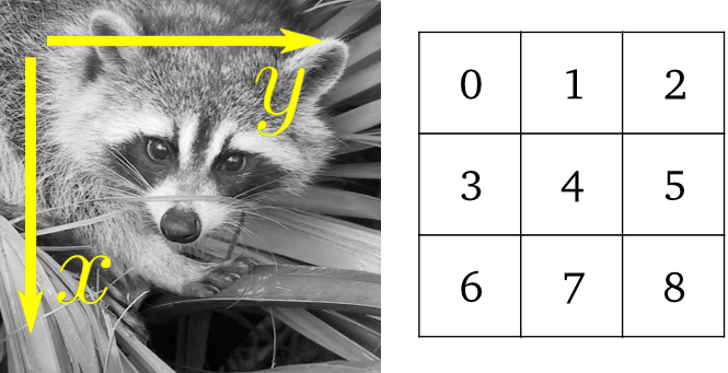
Image = 2-D numerical array

(or 3-D: CT, MRI, 2D + time; 4-D, ...)

Here, image == Numpy array np.array

Tools used in this tutorial:

• numpy: basic array manipulation

• scipy: scipy.ndimage submodule dedicated to image processing (n-dimensional images). Seehttp://docs.scipy.org/doc/scipy/reference/tutorial/ndimage.html

  >>>

  >>> from scipy import ndimage
  

Common tasks in image processing:

• Input/Output, displaying images
• Basic manipulations: cropping, flipping, rotating, ...
• Image filtering: denoising, sharpening
• Image segmentation: labeling pixels corresponding to different objects
• Classification
• Feature extraction
• Registration
• ...

More powerful and complete modules:

• OpenCV (Python bindings)
• CellProfiler
• ITK with Python bindings
• many more...

Chapters contents

• Opening and writing to image files
• Displaying images
• Basic manipulations
  • Statistical information
  • Geometrical transformations
• Image filtering
  • Blurring/smoothing
  • Sharpening
  • Denoising
  • Mathematical morphology
• Feature extraction
  • Edge detection
  • Segmentation
• Measuring objects properties: ndimage.measurements

2.6.1. Opening and writing to image files

Writing an array to a file:

from scipy import misc
l = misc.lena()
misc.imsave('lena.png', l) # uses the Image module (PIL)
import matplotlib.pyplot as plt
plt.imshow(l)
plt.show()

Creating a numpy array from an image file:

>>>

>>> from scipy import misc
>>> lena = misc.imread('lena.png')
>>> type(lena)
<type 'numpy.ndarray'>
>>> lena.shape, lena.dtype
((512, 512), dtype('uint8'))

dtype is uint8 for 8-bit images (0-255)

Opening raw files (camera, 3-D images)

>>>

>>> l.tofile('lena.raw') # Create raw file
>>> lena_from_raw = np.fromfile('lena.raw', dtype=np.int64)
>>> lena_from_raw.shape
(262144,)
>>> lena_from_raw.shape = (512, 512)
>>> import os
>>> os.remove('lena.raw')

Need to know the shape and dtype of the image (how to separate data bytes).

For large data, use np.memmap for memory mapping:

>>>

>>> lena_memmap = np.memmap('lena.raw', dtype=np.int64, shape=(512, 512))

(data are read from the file, and not loaded into memory)

Working on a list of image files

>>>

>>> for i in range(10):
...     im = np.random.random_integers(0, 255, 10000).reshape((100, 100))
...     misc.imsave('random_%02d.png' % i, im)
>>> from glob import glob
>>> filelist = glob('random*.png')
>>> filelist.sort()

2.6.2. Displaying images

Use matplotlib and imshow to display an image inside a matplotlib figure:

>>>

>>> l = misc.lena()
>>> import matplotlib.pyplot as plt
>>> plt.imshow(l, cmap=plt.cm.gray)
<matplotlib.image.AxesImage object at 0x3c7f710>

Increase contrast by setting min and max values:

>>>

>>> plt.imshow(l, cmap=plt.cm.gray, vmin=30, vmax=200)
<matplotlib.image.AxesImage object at 0x33ef750>
>>> # Remove axes and ticks
>>> plt.axis('off')
(-0.5, 511.5, 511.5, -0.5)

Draw contour lines:

>>>

>>> plt.contour(l, [60, 211])
<matplotlib.contour.ContourSet instance at 0x33f8c20>

[Python source code]

For fine inspection of intensity variations, use interpolation='nearest':

>>>

>>> plt.imshow(l[200:220, 200:220], cmap=plt.cm.gray)
>>> plt.imshow(l[200:220, 200:220], cmap=plt.cm.gray, interpolation='nearest')

[Python source code]

3-D visualization: Mayavi

See 3D plotting with Mayavi.

• Image plane widgets
• Isosurfaces
• ...

2.6.3. Basic manipulations

Images are arrays: use the whole numpy machinery.

>>>

>>> lena = scipy.misc.lena()
>>> lena[0, 40]
166
>>> # Slicing
>>> lena[10:13, 20:23]
array([[158, 156, 157],
[157, 155, 155],
[157, 157, 158]])
>>> lena[100:120] = 255
>>>
>>> lx, ly = lena.shape
>>> X, Y = np.ogrid[0:lx, 0:ly]
>>> mask = (X - lx / 2) ** 2 + (Y - ly / 2) ** 2 > lx * ly / 4
>>> # Masks
>>> lena[mask] = 0
>>> # Fancy indexing
>>> lena[range(400), range(400)] = 255

[Python source code]

2.6.3.1. Statistical information

>>>

>>> lena = misc.lena()
>>> lena.mean()
124.04678344726562
>>> lena.max(), lena.min()
(245, 25)

np.histogram

Exercise

• Open as an array the scikit-image logo (http://scikit-image.org/_static/scikits_image_logo.png), or an image that you have on your computer.
• Crop a meaningful part of the image, for example the python circle in the logo.
• Display the image array using matlplotlib. Change the interpolation method and zoom to see the difference.
• Transform your image to greyscale
• Increase the contrast of the image by changing its minimum and maximum values. Optional: use scipy.stats.scoreatpercentile (read the docstring!) to saturate 5% of the darkest pixels and 5% of the lightest pixels.
• Save the array to two different file formats (png, jpg, tiff)

2.6.3.2. Geometrical transformations

>>>

>>> lena = misc.lena()
>>> lx, ly = lena.shape
>>> # Cropping
>>> crop_lena = lena[lx / 4: - lx / 4, ly / 4: - ly / 4]
>>> # up <-> down flip
>>> flip_ud_lena = np.flipud(lena)
>>> # rotation
>>> rotate_lena = ndimage.rotate(lena, 45)
>>> rotate_lena_noreshape = ndimage.rotate(lena, 45, reshape=False)

[Python source code]

2.6.4. Image filtering

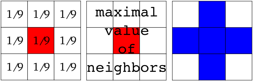
Local filters: replace the value of pixels by a function of the values of neighboring pixels.

Neighbourhood: square (choose size), disk, or more complicated structuring element.

2.6.4.1. Blurring/smoothing

Gaussian filter from scipy.ndimage:

>>>

>>> from scipy import misc
>>> lena = misc.lena()
>>> blurred_lena = ndimage.gaussian_filter(lena, sigma=3)
>>> very_blurred = ndimage.gaussian_filter(lena, sigma=5)

Uniform filter

>>>

>>> local_mean = ndimage.uniform_filter(lena, size=11)

[Python source code]

2.6.4.2. Sharpening

Sharpen a blurred image:

>>>

>>> from scipy import misc
>>> lena = misc.lena()
>>> blurred_l = ndimage.gaussian_filter(lena, 3)

increase the weight of edges by adding an approximation of the Laplacian:

>>>

>>> filter_blurred_l = ndimage.gaussian_filter(blurred_l, 1)
>>> alpha = 30
>>> sharpened = blurred_l + alpha * (blurred_l - filter_blurred_l)

[Python source code]

2.6.4.3. Denoising

Noisy lena:

>>>

>>> from scipy import misc
>>> l = misc.lena()
>>> l = l[230:310, 210:350]
>>> noisy = l + 0.4 * l.std() * np.random.random(l.shape)

A Gaussian filter smoothes the noise out... and the edges as well:

>>>

>>> gauss_denoised = ndimage.gaussian_filter(noisy, 2)

Most local linear isotropic filters blur the image (ndimage.uniform_filter)

A median filter preserves better the edges:

>>>

>>> med_denoised = ndimage.median_filter(noisy, 3)

[Python source code]

Median filter: better result for straight boundaries (low curvature):

>>>

>>> im = np.zeros((20, 20))
>>> im[5:-5, 5:-5] = 1
>>> im = ndimage.distance_transform_bf(im)
>>> im_noise = im + 0.2 * np.random.randn(*im.shape)
>>> im_med = ndimage.median_filter(im_noise, 3)

[Python source code]

Other rank filter: ndimage.maximum_filter, ndimage.percentile_filter

Other local non-linear filters: Wiener (scipy.signal.wiener), etc.

Non-local filters

Exercise: denoising

• Create a binary image (of 0s and 1s) with several objects (circles, ellipses, squares, or random shapes).
• Add some noise (e.g., 20% of noise)
• Try two different denoising methods for denoising the image: gaussian filtering and median filtering.
• Compare the histograms of the two different denoised images. Which one is the closest to the histogram of the original (noise-free) image?

2.6.4.4. Mathematical morphology

See http://en.wikipedia.org/wiki/Mathematical_morphology

Probe an image with a simple shape (a structuring element), and modify this image according to how the shape locally fits or misses the image.

Structuring element:

>>>

>>> el = ndimage.generate_binary_structure(2, 1)
>>> el
array([[False,  True, False],
       [ True,  True,  True],
       [False,  True, False]], dtype=bool)
>>> el.astype(np.int)
array([[0, 1, 0],
       [1, 1, 1],
       [0, 1, 0]])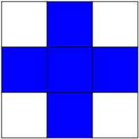

Erosion = minimum filter. Replace the value of a pixel by the minimal value covered by the structuring element.:

>>>

>>> a = np.zeros((7,7), dtype=np.int)
>>> a[1:6, 2:5] = 1
>>> a
array([[0, 0, 0, 0, 0, 0, 0],
       [0, 0, 1, 1, 1, 0, 0],
       [0, 0, 1, 1, 1, 0, 0],
       [0, 0, 1, 1, 1, 0, 0],
       [0, 0, 1, 1, 1, 0, 0],
       [0, 0, 1, 1, 1, 0, 0],
       [0, 0, 0, 0, 0, 0, 0]])
>>> ndimage.binary_erosion(a).astype(a.dtype)
array([[0, 0, 0, 0, 0, 0, 0],
       [0, 0, 0, 0, 0, 0, 0],
       [0, 0, 0, 1, 0, 0, 0],
       [0, 0, 0, 1, 0, 0, 0],
       [0, 0, 0, 1, 0, 0, 0],
       [0, 0, 0, 0, 0, 0, 0],
       [0, 0, 0, 0, 0, 0, 0]])
>>> #Erosion removes objects smaller than the structure
>>> ndimage.binary_erosion(a, structure=np.ones((5,5))).astype(a.dtype)
array([[0, 0, 0, 0, 0, 0, 0],
       [0, 0, 0, 0, 0, 0, 0],
       [0, 0, 0, 0, 0, 0, 0],
       [0, 0, 0, 0, 0, 0, 0],
       [0, 0, 0, 0, 0, 0, 0],
       [0, 0, 0, 0, 0, 0, 0],
       [0, 0, 0, 0, 0, 0, 0]])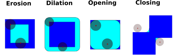

Dilation: maximum filter:

>>>

>>> a = np.zeros((5, 5))
>>> a[2, 2] = 1
>>> a
array([[ 0.,  0.,  0.,  0.,  0.],
       [ 0.,  0.,  0.,  0.,  0.],
       [ 0.,  0.,  1.,  0.,  0.],
       [ 0.,  0.,  0.,  0.,  0.],
       [ 0.,  0.,  0.,  0.,  0.]])
>>> ndimage.binary_dilation(a).astype(a.dtype)
array([[ 0.,  0.,  0.,  0.,  0.],
       [ 0.,  0.,  1.,  0.,  0.],
       [ 0.,  1.,  1.,  1.,  0.],
       [ 0.,  0.,  1.,  0.,  0.],
       [ 0.,  0.,  0.,  0.,  0.]])

Also works for grey-valued images:

>>>

>>> np.random.seed(2)
>>> x, y = (63*np.random.random((2, 8))).astype(np.int)
>>> im[x, y] = np.arange(8)
>>> bigger_points = ndimage.grey_dilation(im, size=(5, 5), structure=np.ones((5, 5)))
>>> square = np.zeros((16, 16))
>>> square[4:-4, 4:-4] = 1
>>> dist = ndimage.distance_transform_bf(square)
>>> dilate_dist = ndimage.grey_dilation(dist, size=(3, 3), \
...         structure=np.ones((3, 3)))

[Python source code]

Opening: erosion + dilation:

>>>

>>> a = np.zeros((5,5), dtype=np.int)
>>> a[1:4, 1:4] = 1; a[4, 4] = 1
>>> a
array([[0, 0, 0, 0, 0],
       [0, 1, 1, 1, 0],
       [0, 1, 1, 1, 0],
       [0, 1, 1, 1, 0],
       [0, 0, 0, 0, 1]])
>>> # Opening removes small objects
>>> ndimage.binary_opening(a, structure=np.ones((3,3))).astype(np.int)
array([[0, 0, 0, 0, 0],
       [0, 1, 1, 1, 0],
       [0, 1, 1, 1, 0],
       [0, 1, 1, 1, 0],
       [0, 0, 0, 0, 0]])
>>> # Opening can also smooth corners
>>> ndimage.binary_opening(a).astype(np.int)
array([[0, 0, 0, 0, 0],
       [0, 0, 1, 0, 0],
       [0, 1, 1, 1, 0],
       [0, 0, 1, 0, 0],
       [0, 0, 0, 0, 0]])

Application: remove noise:

>>>

>>> square = np.zeros((32, 32))
>>> square[10:-10, 10:-10] = 1
>>> np.random.seed(2)
>>> x, y = (32*np.random.random((2, 20))).astype(np.int)
>>> square[x, y] = 1
>>> open_square = ndimage.binary_opening(square)
>>> eroded_square = ndimage.binary_erosion(square)
>>> reconstruction = ndimage.binary_propagation(eroded_square, mask=square)

[Python source code]

Closing: dilation + erosion

Many other mathematical morphology operations: hit and miss transform, tophat, etc.

2.6.5. Feature extraction

2.6.5.1. Edge detection

Synthetic data:

>>>

>>> im = np.zeros((256, 256))
>>> im[64:-64, 64:-64] = 1
>>>
>>> im = ndimage.rotate(im, 15, mode='constant')
>>> im = ndimage.gaussian_filter(im, 8)

Use a gradient operator (Sobel) to find high intensity variations:

>>>

>>> sx = ndimage.sobel(im, axis=0, mode='constant')
>>> sy = ndimage.sobel(im, axis=1, mode='constant')
>>> sob = np.hypot(sx, sy)

[Python source code]

2.6.5.2. Segmentation

• Histogram-based segmentation (no spatial information)

>>>

>>> n = 10
>>> l = 256
>>> im = np.zeros((l, l))
>>> np.random.seed(1)
>>> points = l*np.random.random((2, n**2))
>>> im[(points[0]).astype(np.int), (points[1]).astype(np.int)] = 1
>>> im = ndimage.gaussian_filter(im, sigma=l/(4.*n))
>>> mask = (im > im.mean()).astype(np.float)
>>> mask += 0.1 * im
>>> img = mask + 0.2*np.random.randn(*mask.shape)
>>> hist, bin_edges = np.histogram(img, bins=60)
>>> bin_centers = 0.5*(bin_edges[:-1] + bin_edges[1:])
>>> binary_img = img > 0.5

[Python source code]

Use mathematical morphology to clean up the result:

>>>

>>> # Remove small white regions
>>> open_img = ndimage.binary_opening(binary_img)
>>> # Remove small black hole
>>> close_img = ndimage.binary_closing(open_img)

[Python source code]

Exercise

Check that reconstruction operations (erosion + propagation) produce a better result than opening/closing:

>>>

>>> eroded_img = ndimage.binary_erosion(binary_img)
>>> reconstruct_img = ndimage.binary_propagation(eroded_img, mask=binary_img)
>>> tmp = np.logical_not(reconstruct_img)
>>> eroded_tmp = ndimage.binary_erosion(tmp)
>>> reconstruct_final = np.logical_not(ndimage.binary_propagation(eroded_tmp, mask=tmp))
>>> np.abs(mask - close_img).mean()
0.014678955078125
>>> np.abs(mask - reconstruct_final).mean()
0.0042572021484375

Exercise

Check how a first denoising step (e.g. with a median filter) modifies the histogram, and check that the resulting histogram-based segmentation is more accurate.

See also

 

More advanced segmentation algorithms are found in the scikit-image: see Scikit-image: image processing.

See also

 

Other Scientific Packages provide algorithms that can be useful for image processing. In this example, we use the spectral clustering function of the scikit-learn in order to segment glued objects.

>>>

>>> from sklearn.feature_extraction import image
>>> from sklearn.cluster import spectral_clustering
>>> l = 100
>>> x, y = np.indices((l, l))
>>> center1 = (28, 24)
>>> center2 = (40, 50)
>>> center3 = (67, 58)
>>> center4 = (24, 70)
>>> radius1, radius2, radius3, radius4 = 16, 14, 15, 14
>>> circle1 = (x - center1[0])**2 + (y - center1[1])**2 < radius1**2
>>> circle2 = (x - center2[0])**2 + (y - center2[1])**2 < radius2**2
>>> circle3 = (x - center3[0])**2 + (y - center3[1])**2 < radius3**2
>>> circle4 = (x - center4[0])**2 + (y - center4[1])**2 < radius4**2
>>> # 4 circles
>>> img = circle1 + circle2 + circle3 + circle4
>>> mask = img.astype(bool)
>>> img = img.astype(float)
>>> img += 1 + 0.2*np.random.randn(*img.shape)
>>> # Convert the image into a graph with the value of the gradient on
>>> # the edges.
>>> graph = image.img_to_graph(img, mask=mask)
>>> # Take a decreasing function of the gradient: we take it weakly
>>> # dependant from the gradient the segmentation is close to a voronoi
>>> graph.data = np.exp(-graph.data/graph.data.std())
>>> labels = spectral_clustering(graph, k=4, mode='arpack')
>>> label_im = -np.ones(mask.shape)
>>> label_im[mask] = labels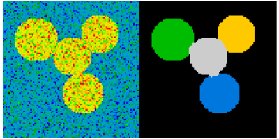

2.6.6. Measuring objects properties:ndimage.measurements

Synthetic data:

>>>

>>> n = 10
>>> l = 256
>>> im = np.zeros((l, l))
>>> points = l*np.random.random((2, n**2))
>>> im[(points[0]).astype(np.int), (points[1]).astype(np.int)] = 1
>>> im = ndimage.gaussian_filter(im, sigma=l/(4.*n))
>>> mask = im > im.mean()

• Analysis of connected components

Label connected components: ndimage.label:

>>>

>>> label_im, nb_labels = ndimage.label(mask)
>>> nb_labels # how many regions?
23
>>> plt.imshow(label_im)        
<matplotlib.image.AxesImage object at ...>

[Python source code]

Compute size, mean_value, etc. of each region:

>>>

>>> sizes = ndimage.sum(mask, label_im, range(nb_labels + 1))
>>> mean_vals = ndimage.sum(im, label_im, range(1, nb_labels + 1))

Clean up small connect components:

>>>

>>> mask_size = sizes < 1000
>>> remove_pixel = mask_size[label_im]
>>> remove_pixel.shape
(256, 256)
>>> label_im[remove_pixel] = 0
>>> plt.imshow(label_im)        
<matplotlib.image.AxesImage object at ...>

Now reassign labels with np.searchsorted:

>>>

>>> labels = np.unique(label_im)
>>> label_im = np.searchsorted(labels, label_im)

[Python source code]

Find region of interest enclosing object:

>>>

>>> slice_x, slice_y = ndimage.find_objects(label_im==4)[0]
>>> roi = im[slice_x, slice_y]
>>> plt.imshow(roi)     
<matplotlib.image.AxesImage object at ...>

[Python source code]

Other spatial measures: ndimage.center_of_mass, ndimage.maximum_position, etc.

Can be used outside the limited scope of segmentation applications.

Example: block mean:

>>>

>>> from scipy import misc
>>> l = misc.lena()
>>> sx, sy = l.shape
>>> X, Y = np.ogrid[0:sx, 0:sy]
>>> regions = sy/6 * (X/4) + Y/6  # note that we use broadcasting
>>> block_mean = ndimage.mean(l, labels=regions, index=np.arange(1,
...     regions.max() +1))
>>> block_mean.shape = (sx/4, sy/6)

[Python source code]

When regions are regular blocks, it is more efficient to use stride tricks (Example: fake dimensions with strides).

Non-regularly-spaced blocks: radial mean:

>>>

>>> sx, sy = l.shape
>>> X, Y = np.ogrid[0:sx, 0:sy]
>>> r = np.hypot(X - sx/2, Y - sy/2)
>>> rbin = (20* r/r.max()).astype(np.int)
>>> radial_mean = ndimage.mean(l, labels=rbin, index=np.arange(1, rbin.max() +1))

[Python source code]

• Other measures

Correlation function, Fourier/wavelet spectrum, etc.

One example with mathematical morphology: granulometry(http://en.wikipedia.org/wiki/Granulometry_%28morphology%29)

>>>

>>> def disk_structure(n):
...     struct = np.zeros((2 * n + 1, 2 * n + 1))
...     x, y = np.indices((2 * n + 1, 2 * n + 1))
...     mask = (x - n)**2 + (y - n)**2 <= n**2
...     struct[mask] = 1
...     return struct.astype(np.bool)
...
>>>
>>> def granulometry(data, sizes=None):
...     s = max(data.shape)
...     if sizes == None:
...         sizes = range(1, s/2, 2)
...     granulo = [ndimage.binary_opening(data, \
...         structure=disk_structure(n)).sum() for n in sizes]
...     return granulo
...
>>>
>>> np.random.seed(1)
>>> n = 10
>>> l = 256
>>> im = np.zeros((l, l))
>>> points = l*np.random.random((2, n**2))
>>> im[(points[0]).astype(np.int), (points[1]).astype(np.int)] = 1
>>> im = ndimage.gaussian_filter(im, sigma=l/(4.*n))
>>>
>>> mask = im > im.mean()
>>>
>>> granulo = granulometry(mask, sizes=np.arange(2, 19, 4))