用pattern进行自然语言处理

http://www.clips.ua.ac.be/pattern

pattern是一个网络数据挖掘的一个工具，分为几个模块

pattern.web 是用来在网络抓取数据的，

pattern.en 是用来处理英文文本的

pattern.search是用来检索特定规律的词汇的 

pattern.vector是用来分类的

pattern.graph用了d3的模块，可以用来可视化展现。

Latent semantic analysis（潜在语义分析）

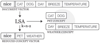
Latent Semantic Analysis (LSA) is a statistical technique based on singular value decomposition (SVD). [1] [2]. It groups related features in the model into concepts (e.g., purr + fur + claw = feline concept). This is called dimensionality reduction. Each document in the model then gets a concept vector, a compressed approximation of the original vector that may be faster for cosine similarity, clustering and classification.

潜在语义分析（LSA）是一个基于奇异值分解的统计方法。它在模型中将相关特征关联成概念（比如咕噜+毛+爪子=猫科 概念）。这被称为降维。模型中的每个文档都有一个概念矩阵，一个对原始向量的近似压缩使得余弦相似度和聚类以及分类算法更快。

SVD requires the Python NumPy package (installed by default on Mac OS X). Given a matrix of documents × features, it yields a matrix U with documents × concepts, a diagonal matrix Σ with singular values, and a matrix Vtwith concepts × features.

SVD要求有NumPy的python包（Mac OS是默认安装的）。给定一个  文档 ×特征 的矩阵，生成U，用奇异值生成对角矩阵Σ，一个矩阵Vt。 

fromnumpy.linalgimportsvd

fromnumpyimportdot, diag

  

u, sigma, vt = svd(matrix, full_matrices=False)

foriinrange(-k,0):

    sigma[i] =0# Reduce k smallest singular values.

 

matrix = dot(u, dot(diag(sigma), vt))

Reference: Wilk J. (2007). http://blog.josephwilk.net/projects/latent-semantic-analysis-in-python.html

The following figure illustrates LSA for a document of words that commonly occur after the word nice:

下面的图表示了LSA，文档中的词在nice后面经常出现的

LSA concept space

The Model.reduce() method calculates SVD and stores the concept space in Model.lsa. The optional dimensions parameter defines the number of dimensions in the concept space: TOP300, L1,L2 (default), an int or a function. There is no universal optimal value, too many dimensions may result in noise while too few may remove useful information.

Model.reduce()函数计算SVD以及在Model.lsa存储概念空间。 可选择的dementions 参数定义了概念空间中的维度的数量：Top 300，L1，L2（默认），一个int或者一个function。没有全局优化值，太多维度可能导致 噪声，太少可能导致信息无用。

When Model.lsa is set, Model.similarity(), neighbors(), search() and cluster() will subsequently compute in LSA concept space. To undo the reduction, set Model.lsa to None. Adding or removing documents in the model will also undo the reduction.

Model.lsa是一个set，Model.similarity(), neighbors(), search() and cluster()在LSA概念空间中紧接着被计算。为了撤销减少，可以设置Model.lsa为None，添加或者删除模型中的文档也会导致降维。

lsa = Model.reduce(dimensions=L2)

lsa = Model.lsa

lsa = LSA(model, k=L2)

lsa.model                  # Parent Model.

lsa.features               # List of features, same as Model.features.

lsa.concepts               # List of concepts, each a {feature: weight} dict.

lsa.vectors                # {Document.id: {concept_index: weight}}

lsa.transform(document)

DimensionsDescriptionTOP300Keep the top 300 dimensions (rule of thumb).L1L1-norm of the singular values as the number of dimensions to remove.L2L2-norm of the singular values as the number of dimensions to remove.intAn int that is the number of dimensions to remove.functionA function that takes the list of singular values and returns an int.

LSA.transform() takes a Document and returns its Vector in concept space. This is useful for documents that are not part of the model – see also Classifier.classify().

LSA.transform() 输入Document 返回概念空间里的Vector 。这对于不在模型中的文档非常有用，同样可以见 Classifier.classify().

The following example demonstrates how related features are grouped after LSA:

以下例子展示的是相关特征怎么被LSA分组

>>>frompattern.vectorimportDocument, Model

>>>

>>> d1 = Document('The cat purrs.', name='cat1')

>>> d2 = Document('Curiosity killed the cat.', name='cat2')

>>> d3 = Document('The dog wags his tail.', name='dog1')

>>> d4 = Document('The dog is happy.', name='dog2')

>>>

>>> m = Model([d1, d2, d3, d4])

>>> m.reduce(2)

>>>

>>>fordinm.documents:

>>>    print

>>>    printd.name

>>>    forconcept, w1inm.lsa.vectors[d.id].items():

>>>        forfeature, w2inm.lsa.concepts[concept].items():

>>>            ifw1 !=0andw2 != 0:

>>>                print(feature, w1 * w2)

The model is reduced to two dimensions. So there are two concepts in the concept space. Each document has a concept vector with weights for each concept. As illustrated below, cat features have been grouped together and dog features have been grouped together.

model减为二维，在概念空间中有两个概念，每个文档都有一个概念向量，向量里面是每个概念的权重，就像下面展示的，猫的概念和狗的概念。（应该0是狗的概念，1是猫的概念吧？）

conceptcatcuriositydoghappykilledpurrstailwags0 0.00 0.00+0.52+0.78 0.00 0.00+0.26+0.261-0.52-0.26 0.00 0.00-0.26-0.78 0.00 0.00conceptd1 (cat1)d2 (cat2)d3 (dog1)d4 (dog2)0 0.00 0.00+0.45+0.901-0.90-0.45 0.00 0.00

Dimensionality reduction is useful with Model.cluster(). Clustering algorithms are exponentially slow (i.e., 3 nested for-loops). Clustering a model of a 1,000 documents with a 1,000 features takes a couple of minutes. However, it takes a couple of seconds to reduce this model to concept vectors with a 100 features, after which k-means clustering also runs in a couple of seconds. Note that document vectors are stored in sparse format (i.e., features with weight 0.0 are omitted), so it is often not necessary to reduce the model. Even if the model has a 1,000 features, each document might have no more than 5-10 features. To get an idea of the average document vector length:

降维对于Model.cluster()非常有用。聚类算法指数降低。聚类一个1000个拥有1000features的文档的model需要几分钟，然而，降维到100概念向量之后只用几秒钟，在降维之后，K-means聚类只用几秒钟。注意到文档向量用稀疏形式存储（比如权重为0的特征被忽略），所以降维也不一定非有必要。

sum(len(d.vector) for d in model.documents) / float(len(model))

Clustering

Clustering is an unsupervised machine learning method that can be used to partition a set of unlabeled documents (i.e., Document objects without a type). Since the label (class, type, category) of a document is not known, clustering will attempt to create clusters (categories) of similar documents by measuring the distance between the document vectors. The optimal solution is then a set of dense clusters, where each cluster is made up of documents with the smallest possible distance between them.

Say we have a number of 2D points with coordinates x and y (horizontal and vertical position). Some points will be further apart than others. The figure below illustrates how we can partition the points by measuring their distance to two centroids. More centroids create more clusters. The principle holds for 3D points with x, y and z coordinates, or any n-D points (x, y, z, ..., n). This is how the k-means clustering algorithm works. A Document.vector is an n-dimensional point. Instead of coordinates x and y it has n features (words) and feature weights. We can calculate the distance between document vectors with cosine similarity.

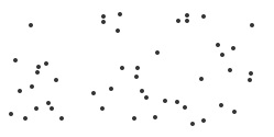random points in 2D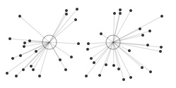points by distance to centroid

The Model.cluster() method returns a list of clusters using the KMEANS or the HIERARCHICAL algorithm. The optional distance parameter can be COSINE (default), EUCLIDEAN, MANHATTAN or HAMMING. An optionaldocuments parameter can be a selective list of documents in the model to cluster.

clusters = Model.cluster(method=KMEANS, k=10, iterations=10, distance=COSINE)

clusters = Model.cluster(method=HIERARCHICAL, k=1, iterations=1000, distance=COSINE)

>>>frompattern.vectorimportDocument, Model, HIERARCHICAL

>>> 

>>> d1 = Document('Cats are independent pets.', name='cat')

>>> d2 = Document('Dogs are trustworthy pets.', name='dog')

>>> d3 = Document('Boxes are made of cardboard.', name='box')

>>> 

>>> m = Model((d1, d2, d3))

>>>printm.cluster(method=HIERARCHICAL, k=2)

 

Cluster([

    Document(id=3, name='box'),

    Cluster([

        Document(id=2, name='dog'),

        Document(id=1, name='cat')

    ])

])

k-means clustering

The k-means clustering algorithm partitions a set of unlabeled documents into k clusters, using k random centroids. It returns a list containing k lists of similar documents. 

Model.cluster(method=KMEANS, k=10, iterations=10, distance=COSINE, seed=RANDOM, p=0.8)

The advantage of k-means is that it is fast. The drawback is that an optimal solution is not guaranteed, since the position of the centroids is random. Each iteration, the algorithm will swap documents between clusters to create denser clusters. 

The optional seed parameter be RANDOM or KMPP. The KMPP or k-means++ initialization algorithm can be used to find better centroids. In many cases this is also faster. The optional parameter p sets the "relaxation" of the k-means algorithm. Relaxation is based on a mathematical trick called triangle inequality, where p=0.5is stable but slow and p=1.0 is prone to errors but faster, especially for higher k and document vectors with many features (i.e., higher dimensionality).

References: 
Arthur, D. (2007). k-means++: the advantages of careful seeding. SODA'07 Proceedings.
Elkan, C. (2003). Using the Triangle Inequality to Accelerate k-Means. ICML'03 Proceedings.

Hierarchical clustering

The hierarchical clustering algorithm returns a tree of nested clusters. The top level item is a Cluster, a mixed list of Document and (nested) Cluster objects.

Model.cluster(method=HIERARCHICAL, k=1, iterations=1000, distance=COSINE)

The advantage of hierarchical clustering is that the optimal solution is guaranteed. Each iteration, the algorithm will cluster the two nearest documents. The drawback is that it is slow.

A Cluster is a list of Document and Cluster objects, with some additional properties:

cluster = Cluster([])

cluster.depth              # Returns the maximum depth of nested clusters.

cluster.flatten(depth=1000)# Returns a flat list, down to the given depth.

cluster.traverse(visit=lambdacluster:None)

>>>frompattern.vectorimportCluster

>>> 

>>> cluster = Cluster((1, Cluster((2, Cluster((3,4))))))

>>>printcluster.depth

>>>printcluster.flatten(1)

 

2

[1,2, Cluster([3,4])]

Note: the maximum recursion depth in Python is 1,000. For deeper clusters, raise sys.setrecursionlimit().

Centroid

The centroid() function takes a Cluster, or a list of Cluster, Document and Vector objects, and returns the mean Vector. The distance() function returns the distance between two vectors. A common problem is that a cluster has no meaningful descriptive name. One solution is to calculate its centroid, and use theDocument.type of the document vector(s) nearest to the centroid.

centroid(vectors=[])           # Returns the mean Vector.

distance(v1, v2, method=COSINE)# COSINE | EUCLIDEAN | MANHATTAN | HAMMING

Classification

分类器

Classification can be used to predict the label of an unlabeled document. More specifically, classification is a supervised machine learning method that uses labeled documents (i.e., Document objects with a type) as training examples to statistically predict the label (class, type) of new documents, based on their similarity to the training examples using a distance metric (e.g., cosine similarity). A Document is a bag-of-words representation of a text, i.e., unordered words + word count. The Document.vector maps the words (or features) to their weight (absolute or relative word count, tf-idf, ...). The weight of a word represents its relevancy in the text. So we can compare how similar two documents are by measuring if they have relevant words in common. Given an unlabeled document, a classifier yields the label of the most similar document(s) in its training set. This implies that a larger training set with more features (and less labels) gives better performance.

分类器能够用来标签未标签的文档。更特别的，分类器是一种监督的机器学习方法，用已经标签的文档（比如Document和type)作为训练集去统计性地预测新文档的标签(class,type)。文档是文本的词袋表示。

For example, if we have a corpus of product reviews (training data) for which the star rating of each product review is known (labels, e.g., ★★★☆☆ = 3), we can use it to predict the star rating of other reviews, based on common words (features) in the text. We could represent each review as a vector of adjectives (e.g., good, bad, awesome, awful, ...) since positive reviews (good, awesome) will most likely contain different adjectives than negative reviews (bad, awful).

The pattern.vector module implements four classification algorithms:

•  NB: Naive Bayes, based on the probability that a feature occurs in a class.
• KNN: k-nearest neighbor, based on the k most similar documents in the training set.
• SLP: single-layer averaged perceptron, based on an artificial neural network.
• SVM: support vector machine, based on a representation of the documents in a high-dimensional space separated by hyperplanes (see further).

classifier =  NB(train=[], baseline=MAJORITY, method=MULTINOMIAL, alpha=0.0001)

classifier = KNN(train=[], baseline=MAJORITY, k=10, distance=COSINE)

classifier = SLP(train=[], baseline=MAJORITY, iterations=1)

classifier = SVM(train=[], type=CLASSIFICATION, kernel=LINEAR)

Classifier

The NB, KNN, SLP and SVM classifiers inherit from the Classifier base class:

classifier = Classifier(train=[], baseline=MAJORITY)

classifier = Classifier.load(path)

classifier.features      # List of trained features (words).

classifier.classes       # List of trained class labels.

classifier.binary        # True if Classifier.classes == [True, False] or [0, 1].

classifier.distribution  # Dictionary of (label, frequency)-items.

classifier.baseline      # Default predicted class (most frequent or user-given).

classifier.majority      # Most frequent class label.

classifier.minority      # Least frequent class label. 

classifier.skewness      # 0.0 if the classes are evenly distributed.

classifier.train(document,type=None)

classifier.classify(document, discrete=True)

classifier.confusion_matrix(documents=[])

classifier.test(documents=[], target=None)

classifier.auc(documents=[], k=10) 

classifier.finalize()    # Trains + removes training data from memory.

classifier.save(path)    # gzipped pickle file, load with Classifier.load().

• Classifier.train() trains the classifier with the given document and type (= class label).
  A document can be a Document, Vector, dict, or a list or string of words (features).
  If no type is given, Document.type will be used instead.
  You can also use Classifier(train=[document1, document2, ...]) with a list or a Model.
• Classifier.classify() returns the type with the highest probability for the given document.
  If discrete=False, returns a dictionary of (class, probability)-items.
  If the classifier is trained on an LSA model, you must supply the output of Model.lsa.transform().
• Classifier.test() returns an (accuracy, precision, recall, F1-score)-tuple.
  The given test data can be a list of documents, (document, type)-tuples or a Model.

Training a classifier

Say we have a corpus of a 1,000 short movie reviews (reviews.csv.zip), each with a star rating given by the reviewer or customer. The corpus contains such instances as:

ReviewRatingAmazing film!★★★★★Pretty darn good★★★★☆Rather disappointing★★☆☆☆How can anyone watch this drivel?☆☆☆☆☆

We can use the corpus to train a classifier that predicts the star rating of other reviews, based on word similarity. By creating a Document for each review we have control over what words (features) are included or not (e.g., stopwords). We will use a Naive Bayes (NB) classifier, but the examples will also work with KNN and SVM, since all classifiers inherit from Classifier.

>>>frompattern.vectorimportDocument, NB

>>>frompattern.dbimportcsv

>>> 

>>> nb = NB()

>>>forreview, rating incsv('reviews.csv'):

>>>     v = Document(review, type=int(rating), stopwords=True)

>>>     nb.train(v)

>>>

>>>printnb.classes

>>>printnb.classify(Document('A good movie!'))

 

[0,1,2,3,4,5]

4

The review "A good movie!" is classified as ★★★★☆ because, based on the training data, the classifier learned that good is often related to higher star ratings.

Testing a classifier

How accurate is the classifier? Naive Bayes can be quite effective despite its simple implementation. In this example it has an accuracy of 60%. Given a set of testing data, NB.test() returns an (accuracy,precision, recall, F1-score)-tuple with values between 0.0–1.0:

NB.test(documents=[], target=None)# Returns (accuracy, precision, recall, F1).

>>> data = csv('reviews.csv')

>>> data = [(review, int(rating))forreview, rating indata]

>>> data = [Document(review, type=rating, stopwords=True)forreview, rating indata]

>>>

>>> nb = NB(train=data[:500])

>>>

>>> accuracy, precision, recall, f1 = nb.test(data[500:])

>>>printaccuracy

 

0.60

Note how we used 1/2 of the data for training and reserve the other 1/2 of the data for testing.

Binary classification

The reported accuracy (60%) is not the worst baseline. Random guessing between the six possible star ratings (0-5) has only 17% accuracy. Moreover, many errors are off by only one (e.g., predicts ★ instead of ★★ or vice versa). If we simplify the task and train a binary classifier that predicts either positive (True → star rating 3, 4, 5) or negative (False → star rating 0, 1, 2), accuracy increases to 68%. This is because we now have only two classes to choose from and more training data per class.

>>> data = csv('reviews.csv')

>>> data = [(review, int(rating) >= 3)forreview, rating indata]

>>> data = [Document(review, type=rating, stopwords=True)forreview, rating indata]

>>>

>>> nb = NB(train=data[:500])

>>>

>>> accuracy, precision, recall, f1 = nb.test(data[500:])

>>>printaccuracy

 

0.68

Skewed data

The reported accuracy can be misleading. Suppose we have a classifier that always predicts positive (True). We evaluate it with a test set that contains 1/2 positive reviews. So accuracy is 50%. We then evaluate it with a test set that contains 9/10 positive reviews. Accuracy is now 90%. This happens if the data is skewed, i.e., when it has more instances of one class and fewer of the other.

A more reliable evaluation is to look at both the rate of correct predictions and incorrect predictions, per class. This information can be derived from the confusion matrix.

Confusion matrix

A ConfusionMatrix is a matrix of actual classes × predicted classes, stored as a dictionary:

confusion = Classifier.confusion_matrix(documents=[])

confusion(target)        # (TP, TN, FP, FN) for given class.

confusion.table          # Pretty string output.

>>>printnb.distribution

>>>printnb.confusion_matrix(data[500:])

>>>printnb.confusion_matrix(data[500:])(True)# (TP, TN, FP, FN)

 

{True:373,False:127}

{True: {True:285,False:94},False: {False:53,True:68}}

(286,53,68,93)

ClassPredicted class TrueFalseTrue28594False6853

The class distribution shows that there are more positive reviews in the training data (373/500).

The confusion matrix shows that, by consequence, the classifier is good at predicting positive reviews (286/373 or 76%) but bad at predicting negative reviews (53/127 or 42%). Note how we call the ConfusionMatrix like a function. This returns a (TP, TN, FP, FN)-tuple for a given class, the amount of true positives ("hits"), true negatives ("rejects"), false positives ("errors") and false negatives ("misses").

下面一个图（来自公开课  https://class.coursera.org/textretrieval-001/wiki/Week1Overview）是自然语言处理的一个处理层次。最底层是lexical analysis,（词法分析，词性标注）。~动词，名词，啥的

在其次是syntactic analysis （parsing）句法分析，从语法上分析。~判别名词短语啥的

pragmatic analysis 语用分析 ~使用场景的分析

semantic analysis 在左边的角落  语义分析，能够分析出来主题和之间的关系，inference是 推断，能够推出man是恐惧的。

 

Sentiment 

语义

Written text can be broadly categorized into two types: facts and opinions. Opinions carry people's sentiments, appraisals and feelings toward the world. The pattern.en module bundles a lexicon of adjectives (e.g., good, bad, amazing, irritating, ...) that occur frequently in product reviews, annotated with scores for sentiment polarity (positive ↔ negative) and subjectivity (objective ↔ subjective). 

书写文本通常能够广义地分成两类，事实和意见。意见带来了人们对世界的情感，评估，感觉。pattern.en 捆绑了经常在产品评论中的形容词，用积极程度和主观程度来评分。

The sentiment() function returns a (polarity, subjectivity)-tuple for the given sentence, based on the adjectives it contains, where polarity is a value between -1.0 and +1.0 and subjectivity between 0.0 and1.0. The sentence can be a string, Text, Sentence, Chunk, Word or a Synset (see below). 

 sentiment() 基于其中的形容词返回 (polarity, subjectivity)元组，polarity 积极程度是-1到1之间以及主观程度是0到1之间。

The positive() function returns True if the given sentence's polarity is above the threshold. The threshold can be lowered or raised, but overall +0.1 gives the best results for product reviews. Accuracy is about 75% for movie reviews.

positive() 在句子的极性在阈值之上的时候返回True，阈值是可以调整的，产品评论最好是0.1，电影评论大概是75%

sentiment(sentence)       # Returns a (polarity, subjectivity)-tuple.

positive(s, threshold=0.1)# Returns True if polarity >= threshold.

>>>frompattern.enimportsentiment

>>> 

>>>printsentiment(

>>>    "The movie attempts to be surreal by incorporating various time paradoxes,"

>>>    "but it's presented in such a ridiculous way it's seriously boring.")

 

(-0.34,1.0)

In the example above, -0.34 is the average of surreal, various, ridiculous and seriously boring. To retrieve the scores for individual words, use the special assessments property, which yields a list of (words,polarity, subjectivity, label)-tuples.

-0.34是形容词的平均值，独立词的召回分析用assessments ，

>>>printsentiment('Wonderfully awful! :-)').assessments

 

[(['wonderfully','awful','!'], -1.0,1.0,None),

 ([':-)'],0.5,1.0,'mood')]

  

---

Mood & modality

Grammatical mood refers to the use of auxiliary verbs (e.g., could, would) and adverbs (e.g., definitely,maybe) to express uncertainty. 

语法上的心情用(could,would)等来表达以及definitely，maybe表达不确定性。

The mood() function returns either INDICATIVE, IMPERATIVE, CONDITIONAL or SUBJUNCTIVE for a given parsed Sentence. See the table below for an overview of moods.

mood() 返回一个句子的 Indicative（陈述），imperative（祈使），conditional（条件），subjnctive（虚拟）

The modality() function returns the degree of certainty as a value between -1.0 and +1.0, where values> +0.5 represent facts. For example, "I wish it would stop raining" scores -0.35, whereas "It will stop raining" scores +0.75. Accuracy is about 68% for Wikipedia texts.

mood(sentence)    # Returns INDICATIVE | IMPERATIVE | CONDITIONAL | SUBJUNCTIVE

modality(sentence)# Returns -1.0 => +1.0.

MoodFormUseExampleINDICATIVEnone of the below fact, beliefIt rains.IMPERATIVEinfinitive without tocommand, warningDon't rain!CONDITIONALwould, could, should, may, or will, can + ifconjectureIt might rain.SUBJUNCTIVEwish, were, or it is + infinitivewish, opinionI hope it rains.

For example:

>>>frompattern.enimportparse, Sentence, parse

>>>frompattern.enimportmodality

>>>

>>> s = "Some amino acids tend to be acidic while others may be basic." # weaseling

>>> s = parse(s, lemmata=True)

>>> s = Sentence(s)

>>>

>>>printmodality(s)

 

0.11

 

Parse trees

A parse tree stores a tagged string as a tree of nested objects that can be traversed to analyze the constituents in the text. The parsetree() function takes the same parameters as parse() and returns aText object. A Text is a list of Sentence objects. Each Sentence is a list of Word objects. Word objects can be grouped in Chunk objects, which are related to other Chunk objects.

parsetree(string,

   tokenize = True,        # Split punctuation marks from words?

       tags = True,        # Parse part-of-speech tags? (NN, JJ, ...)

     chunks = True,        # Parse chunks? (NP, VP, PNP, ...)

  relations = False,       # Parse chunk relations? (-SBJ, -OBJ, ...)

    lemmata = False,       # Parse lemmata? (ate => eat)

   encoding = 'utf-8'      # Input string encoding.

     tagset = None)        # Penn Treebank II (default) or UNIVERSAL.

The following example shows the parse tree for the sentence "The cat sat on the mat.":

>>>frompattern.enimportparsetree

>>>

>>> s = parsetree('The cat sat on the mat.', relations=True, lemmata=True)

>>>printrepr(s)

 

[Sentence(

 u'The/DT/B-NP/O/NP-SBJ-1/the

   cat/NN/I-NP/O/NP-SBJ-1/cat

   sat/VBD/B-VP/O/VP-1/sit

   on/IN/B-PP/B-PNP/O/on

   the/DT/B-NP/I-PNP/O/the

   mat/NN/I-NP/I-PNP/O/mat

   ././O/O/O/O/.')]

>>>forsentenceins:

>>>    forchunkinsentence.chunks:

>>>        printchunk.type, [(w.string, w.type)forwinchunk.words]

 

NP [(u'the', u'DT'), (u'cat', u'NN')]

VP [(u'sat', u'VBD')]

PP [(u'on', u'IN')]

NP [(u'the','DT), (u'mat', u'NN')]

A common approach is to store output from parse() in a .txt file, with a tagged sentence on each line. Thetree() function can be used to load it as a Text object. It has an optional token parameter that defines the format of the tokens (tagged words). So parsetree(s) is the same as tree(parse(s)).

tree(taggedstring, token=[WORD, POS, CHUNK, PNP, REL, LEMMA])

>>>frompattern.enimporttree

>>>

>>>forsentenceintree(open('tagged.txt'), token=[WORD, POS, CHUNK])

>>>    printsentence