OpenCV,三大边缘检测Canny,Sobel,Laplacian,及MFC实现
来源:互联网 发布:淘宝信誉查询 编辑:程序博客网 时间:2024/05/29 19:36
本文部分文字Copy自OpenCV中文网站
Sobel
使用扩展 Sobel 算子计算一阶、二阶、三阶或混合图像差分
void cvSobel( const CvArr* src, CvArr* dst, int xorder, int yorder, int aperture_size=3 );
- src
- 输入图像.
- dst
- 输出图像.
- xorder
- x 方向上的差分阶数
- yorder
- y 方向上的差分阶数
- aperture_size
- 扩展 Sobel 核的大小,必须是 1, 3, 5 或 7。 除了尺寸为 1, 其它情况下, aperture_size ×aperture_size 可分离内核将用来计算差分。对 aperture_size=1的情况, 使用 3x1 或 1x3 内核 (不进行高斯平滑操作)。这里有一个特殊变量 CV_SCHARR (=-1),对应 3x3 Scharr 滤波器,可以给出比 3x3 Sobel 滤波更精确的结果。Scharr 滤波器系数是:

- 对 x-方向 或矩阵转置后对 y-方向。
函数 cvSobel 通过对图像用相应的内核进行卷积操作来计算图像差分:

由于Sobel 算子结合了 Gaussian 平滑和微分,所以,其结果或多或少对噪声有一定的鲁棒性。通常情况,函数调用采用如下参数 (xorder=1, yorder=0, aperture_size=3) 或 (xorder=0, yorder=1, aperture_size=3) 来计算一阶 x- 或 y- 方向的图像差分。第一种情况对应:
 核。
核。
第二种对应:

或者

核的选则依赖于图像原点的定义 (origin 来自 IplImage 结构的定义)。由于该函数不进行图像尺度变换,所以和输入图像(数组)相比,输出图像(数组)的元素通常具有更大的绝对数值(译者注:即像素的位深)。为防止溢出,当输入图像是 8 位的,要求输出图像是 16 位的。当然可以用函数 cvConvertScale 或 cvConvertScaleAbs 把运算结果(dst)转换为 8 位的。除了8-位图像,函数也接受 32-位 浮点数图像。所有输入和输出图像都必须是单通道的,并且具有相同的图像尺寸或者ROI尺寸。
Sobel原理
Note
以下内容来自于Bradski和Kaehler的大作: Learning OpenCV .
上面两节我们已经学习了卷积操作。一个最重要的卷积运算就是导数的计算(或者近似计算).
为什么对图像进行求导是重要的呢? 假设我们需要检测图像中的 边缘 ,如下图:
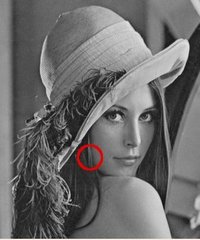
你可以看到在 边缘 ,相素值显著的 改变 了。表示这一 改变 的一个方法是使用 导数 。 梯度值的大变预示着图像中内容的显著变化。
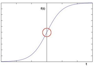
用更加形象的图像来解释,假设我们有一张一维图形。下图中灰度值的”跃升”表示边缘的存在:
使用一阶微分求导我们可以更加清晰的看到边缘”跃升”的存在(这里显示为高峰值)
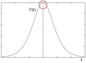
从上例中我们可以推论检测边缘可以通过定位梯度值大于邻域的相素的方法找到(或者推广到大于一个阀值).
更加详细的解释,请参考Bradski 和 Kaehler的 Learning OpenCV 。
Sobel算子
- Sobel 算子是一个离散微分算子 (discrete differentiation operator)。 它用来计算图像灰度函数的近似梯度。
- Sobel 算子结合了高斯平滑和微分求导。
计算
假设被作用图像为  :
:
在两个方向求导:
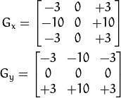
水平变化: 将
与一个奇数大小的内核  进行卷积。比如,当内核大小为3时, 的计算结果为:
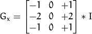
垂直变化: 将:math:I 与一个奇数大小的内核
 进行卷积。比如,当内核大小为3时, 的计算结果为:
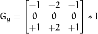
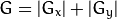
在图像的每一点,结合以上两个结果求出近似 梯度:
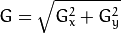
有时也用下面更简单公式代替:
Note
当内核大小为
时, 以上Sobel内核可能产生比较明显的误差(毕竟,Sobel算子只是求取了导数的近似值)。 为解决这一问题,OpenCV提供了Scharr 函数,但该函数仅作用于大小为3的内核。该函数的运算与Sobel函数一样快,但结果却更加精确,其内核为:
关于( Scharr )的更多信息请参考OpenCV文档。在下面的示例代码中,你会发现在 Sobel 函数调用的上面有被注释掉的 Scharr 函数调用。 反注释Scharr调用 (当然也要相应的注释掉Sobel调用),看看该函数是如何工作的。
源码
- 本程序做什么?
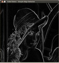
- 使用 Sobel算子 产生的输出图像上,检测到的亮起的 边缘 相素散布在更暗的背景中。
- 下面是本教程的源码,你也可以从 here 下载
解释
首先申明变量:
装载原图像 src:
第一步对原图像使用 GaussianBlur 降噪 ( 内核大小 = 3 )
将降噪后的图像转换为灰度图:
第二步,在 x 和 y 方向分别”求导“。 为此,我们使用函数 Sobel :
该函数接受了以下参数:
- src_gray: 在本例中为输入图像,元素类型 CV_8U
- grad_x/grad_y: 输出图像.
- ddepth: 输出图像的深度,设定为 CV_16S 避免外溢。
- x_order: x 方向求导的阶数。
- y_order: y 方向求导的阶数。
- scale, delta 和 BORDER_DEFAULT: 使用默认值
注意为了在 x 方向求导我们使用:
 ,
,  . 采用同样方法在 y 方向求导。
将中间结果转换到 CV_8U:
将两个方向的梯度相加来求取近似 梯度 (注意这里没有准确的计算,但是对我们来讲已经足够了)。
最后,显示结果:
结果
这里是将Sobel算子作用于 lena.jpg 的结果:
Laplace
计算图像的 Laplacian 变换
void cvLaplace( const CvArr* src, CvArr* dst, int aperture_size=3 );
- src
- 输入图像.
- dst
- 输出图像.
- aperture_size
- 核大小 (与 cvSobel 中定义一样).
函数 cvLaplace 计算输入图像的 Laplacian变换,方法是先用 sobel 算子计算二阶 x- 和 y- 差分,再求和:

对 aperture_size=1 则给出最快计算结果,相当于对图像采用如下内核做卷积:

类似于 cvSobel 函数,该函数也不作图像的尺度变换,所支持的输入、输出图像类型的组合和cvSobel一致。
Canny
采用 Canny 算法做边缘检测
void cvCanny( const CvArr* image, CvArr* edges, double threshold1, double threshold2, int aperture_size=3 );
- image
- 单通道输入图像.
- edges
- 单通道存储边缘的输出图像
- threshold1
- 第一个阈值
- threshold2
- 第二个阈值
- aperture_size
- Sobel 算子内核大小 (见 cvSobel).
函数 cvCanny 采用 CANNY 算法发现输入图像的边缘而且在输出图像中标识这些边缘。threshold1和threshold2 当中的小阈值用来控制边缘连接,大的阈值用来控制强边缘的初始分割。
1,Sobel与Scharr算子
<span style="font-size:12px;">// ConsoleAppOpenCVSobel.cpp : Defines the entry point for the console application.//#include "stdafx.h"/** * @file Sobel_Demo.cpp * @brief Sample code using Sobel and/or Scharr OpenCV functions to make a simple Edge Detector * @author OpenCV team */#include "opencv2/imgproc/imgproc.hpp"#include "opencv2/highgui/highgui.hpp"#include <stdlib.h>#include <stdio.h>#include "iostream"using namespace cv;using namespace std;/** * @function main *//** Global Variables */ const int alpha_slider_max = 100;//滑动条最大值 int alpha_slider_init=10;//滑动条初始值 double alpha; double beta; /** Matrices to store images */ Mat abs_grad_x;//第一附图 Mat abs_grad_y;//第二幅图 Mat dst;//存储融合后的图像 static void on_trackbar( int, void* ) { //判断两幅图片是否相同以及是否成功读入 CV_Assert(abs_grad_x.depth() == CV_8U); CV_Assert(abs_grad_x.depth() == abs_grad_y.depth()); CV_Assert(abs_grad_x.size() == abs_grad_y.size()); if( !abs_grad_x.data ) cout<<"Error loading src1"<<endl; if( !abs_grad_y.data ) cout<<"Error loading src2"<<endl; /******************融合开始********************/ alpha = (double) alpha_slider_init/alpha_slider_max ; beta = ( 1.0 - alpha ); addWeighted( abs_grad_x, alpha, abs_grad_y, beta, 0.0, dst);//线性融合 imshow( "Linear Blend", dst ); } int _tmain(int argc, _TCHAR* argv[]){ Mat src, src_gray; Mat grad; const char* TrackbarName = "Sobel Demo - Simple Edge Detector"; int scale = 1; int delta = 0; int ddepth = CV_16S; /// Load an image src = imread( "building.jpg" ); if( !src.data ) { return -1; } GaussianBlur( src, src, Size(3,3), 0, 0, BORDER_DEFAULT ); /// Convert it to gray cvtColor( src, src_gray, COLOR_RGB2GRAY );//转换图像为灰度图 /// Create window namedWindow( TrackbarName, WINDOW_AUTOSIZE ); /// Generate grad_x and grad_y Mat grad_x, grad_y; //Mat abs_grad_x, abs_grad_y; /// Gradient X(X梯度) //对图像x方向进行一阶差分,得到的图像垂直的边缘比较明显 //Scharr( src_gray, grad_x, ddepth, 1, 0, scale, delta, BORDER_DEFAULT ); Sobel( src_gray, grad_x, ddepth, 1, 0, 3, scale, delta, BORDER_DEFAULT ); convertScaleAbs( grad_x, abs_grad_x );//转换数组元素成8位无符号整型 /// Gradient Y(Y梯度) //对图像y方向进行一阶差分,得到的图像水平的边缘比较明显 //Scharr( src_gray, grad_y, ddepth, 0, 1, scale, delta, BORDER_DEFAULT ); Sobel( src_gray, grad_y, ddepth, 0, 1, 3, scale, delta, BORDER_DEFAULT ); convertScaleAbs( grad_y, abs_grad_y ); /// Total Gradient (approximate)(总梯度),并创建滑动条 /// Create Windows namedWindow("Linear Blend", 1); /// 创建滑动条 createTrackbar( TrackbarName, "Linear Blend", &alpha_slider_init, alpha_slider_max, on_trackbar ); /// Show some stuff on_trackbar( alpha_slider_init, 0 ); waitKey(0); return 0;}</span>


二,OpenCV+MFC简单实现


- OpenCV,三大边缘检测Canny,Sobel,Laplacian,及MFC实现
- opencv边缘检测(robert,prewitt,sobel,canny,laplacian)
- [学习opencv]图像sobel、laplacian、canny边缘检测
- Android opencv(三) 边缘检测Sobel、Canny
- 图像sobel、laplacian、canny边缘检测算法基础实现
- vim+python+OpenCV学习七 : Sobel算子、Laplacian算子和Canny边缘检测
- OpenCV-Python教程(6)(7)(8): Sobel算子 Laplacian算子 Canny边缘检测
- opencv的Sobel导数、Scharr滤波器、Laplacian算子、Canny边缘检测
- opencv3学习之边缘检测(Canny/Sobel/Laplacian算子)
- opencv边缘检测Sobel和Canny
- opencv实现sobel边缘检测
- OpenCV 实现canny边缘检测
- 基于OpenCV的canny边缘检测的MFC实现
- OpenCV笔记:图像边缘检测Sobel,Laplace,Canny
- 使用OpenCV对图像作边缘检测(Canny、Sobel、Laplace)
- canny/Sobel/Laplace边缘检测
- 图像处理中各种边缘检测的微分算子简单比较(Sobel,Robert, Prewitt,Laplacian,Canny)
- 图像处理中各种边缘检测的微分算子简单比较(Sobel,Robert, Prewitt,Laplacian,Canny)
- CSS Hack技术详解,支持IE 6-11、Chrome、FireFox、Safari、Opera
- HTTP协议header头域
- 安卓预置APK
- PHP实现在指定数组中取指定数量不重复的子集合
- 欧几里德算法求最大公约数
- OpenCV,三大边缘检测Canny,Sobel,Laplacian,及MFC实现
- 福源灏:300粉丝,微盟旺铺单日成交额39万
- 跨域文件clientaccesspolicy.xml
- boost的shared_ptr循环引用
- 【BZOJ 3218】 a + b Problem
- (转载)Android数据库高手秘籍(二)——创建表和LitePal的基本用法
- 8个炫酷的HTML5动画、应用和游戏
- SDUTOJ 2074 区间覆盖问题 贪心
- 外交部就李克强总理出席世界经济论坛2015年年会举行中外媒体吹风会