深度学习基础（五）Softmax Regression

来源：互联网发布：日语汉字读音软件编辑：程序博客网时间：2024/04/30 19:20

Softmax Regression

Softmax Regression是 Logistic Regression的推广

假设我们有训练集 $\{ (x^{(1)}, y^{(1)}), \ldots, (x^{(m)}, y^{(m)}) \}$

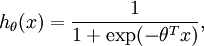
Logistic Regression:

对于每个特征 $x^{(i)} \in \Re^{n+1}$ ，标签 $y^{(i)} \in \{0,1\}$

$\begin{align}h_\theta(x) = \frac{1}{1+\exp(-\theta^Tx)},\end{align}$

$\begin{align}J(\theta) = -\frac{1}{m} \left[ \sum_{i=1}^m y^{(i)} \log h_\theta(x^{(i)}) + (1-y^{(i)}) \log (1-h_\theta(x^{(i)})) \right]\end{align}$

$\begin{align}J(\theta) &= -\frac{1}{m} \left[ \sum_{i=1}^m (1-y^{(i)}) \log (1-h_\theta(x^{(i)})) + y^{(i)} \log h_\theta(x^{(i)}) \right] \\&= - \frac{1}{m} \left[ \sum_{i=1}^{m} \sum_{j=0}^{1} 1\left\{y^{(i)} = j\right\} \log p(y^{(i)} = j | x^{(i)} ; \theta) \right]\end{align}$

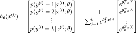
Softmax Regression:

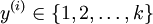
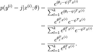
对于每个特征 $x^{(i)} \in \Re^{n+1}$ ，标签 $y^{(i)} \in \{1, 2, \ldots, k\}$

$\begin{align}h_\theta(x^{(i)}) =\begin{bmatrix}p(y^{(i)} = 1 | x^{(i)}; \theta) \\p(y^{(i)} = 2 | x^{(i)}; \theta) \\\vdots \\p(y^{(i)} = k | x^{(i)}; \theta)\end{bmatrix}=\frac{1}{ \sum_{j=1}^{k}{e^{ \theta_j^T x^{(i)} }} }\begin{bmatrix}e^{ \theta_1^T x^{(i)} } \\e^{ \theta_2^T x^{(i)} } \\\vdots \\e^{ \theta_k^T x^{(i)} } \\\end{bmatrix}\end{align}$

$\begin{align}J(\theta) = - \frac{1}{m} \left[ \sum_{i=1}^{m} \sum_{j=1}^{k} 1\left\{y^{(i)} = j\right\} \log \frac{e^{\theta_j^T x^{(i)}}}{\sum_{l=1}^k e^{ \theta_l^T x^{(i)} }}\right]\end{align}$

Softmax Regression有一个很特别地性质：过参数化

$\begin{align}p(y^{(i)} = j | x^{(i)} ; \theta)&= \frac{e^{(\theta_j-\psi)^T x^{(i)}}}{\sum_{l=1}^k e^{ (\theta_l-\psi)^T x^{(i)}}} \\&= \frac{e^{\theta_j^T x^{(i)}} e^{-\psi^Tx^{(i)}}}{\sum_{l=1}^k e^{\theta_l^T x^{(i)}} e^{-\psi^Tx^{(i)}}} \\&= \frac{e^{\theta_j^T x^{(i)}}}{\sum_{l=1}^k e^{ \theta_l^T x^{(i)}}}.\end{align}$

可以看到参数减去任意的一个值并不影响我们的假设，也就是说有很多歌参数满足我们的假设

为了避免过大参数的影响，

$\begin{align}J(\theta) = - \frac{1}{m} \left[ \sum_{i=1}^{m} \sum_{j=1}^{k} 1\left\{y^{(i)} = j\right\} \log \frac{e^{\theta_j^T x^{(i)}}}{\sum_{l=1}^k e^{ \theta_l^T x^{(i)} }} \right] + \frac{\lambda}{2} \sum_{i=1}^k \sum_{j=0}^n \theta_{ij}^2\end{align}$

$\begin{align}\nabla_{\theta_j} J(\theta) = - \frac{1}{m} \sum_{i=1}^{m}{ \left[ x^{(i)} ( 1\{ y^{(i)} = j\} - p(y^{(i)} = j | x^{(i)}; \theta) ) \right] } + \lambda \theta_j\end{align}$

参考练习：

http://deeplearning.stanford.edu/wiki/index.php/Exercise:Softmax_Regression

实验步骤：

0. 初始化参数和常亮

1.载入数据

2.计算代价函数

3.Gradient checking

4.训练

5.测试

%% CS294A/CS294W Softmax Exercise %  Instructions%  ------------% %  This file contains code that helps you get started on the%  softmax exercise. You will need to write the softmax cost function %  in softmaxCost.m and the softmax prediction function in softmaxPred.m. %  For this exercise, you will not need to change any code in this file,%  or any other files other than those mentioned above.%  (However, you may be required to do so in later exercises)%%======================================================================%% STEP 0: Initialise constants and parameters%%  Here we define and initialise some constants which allow your code%  to be used more generally on any arbitrary input. %  We also initialise some parameters used for tuning the model.inputSize = 28 * 28; % Size of input vector (MNIST images are 28x28)numClasses = 10;     % Number of classes (MNIST images fall into 10 classes)lambda = 1e-4; % Weight decay parameter%%======================================================================%% STEP 1: Load data%%  In this section, we load the input and output data.%  For softmax regression on MNIST pixels, %  the input data is the images, and %  the output data is the labels.%% Change the filenames if you've saved the files under different names% On some platforms, the files might be saved as % train-images.idx3-ubyte / train-labels.idx1-ubyteimages = loadMNISTImages('train-images-idx3-ubyte');labels = loadMNISTLabels('train-labels-idx1-ubyte');labels(labels==0) = 10; % Remap 0 to 10inputData = images;% For debugging purposes, you may wish to reduce the size of the input data% in order to speed up gradient checking. % Here, we create synthetic dataset using random data for testingDEBUG = true; % Set DEBUG to true when debugging.if DEBUG    inputSize = 8;    inputData = randn(8, 100);    labels = randi(10, 100, 1);end% Randomly initialise thetatheta = 0.005 * randn(numClasses * inputSize, 1);%%======================================================================%% STEP 2: Implement softmaxCost%%  Implement softmaxCost in softmaxCost.m. [cost, grad] = softmaxCost(theta, numClasses, inputSize, lambda, inputData, labels);                                     %%======================================================================%% STEP 3: Gradient checking%%  As with any learning algorithm, you should always check that your%  gradients are correct before learning the parameters.% if DEBUG    numGrad = computeNumericalGradient( @(x) softmaxCost(x, numClasses, ...                                    inputSize, lambda, inputData, labels), theta);    % Use this to visually compare the gradients side by side    disp([numGrad grad]);     % Compare numerically computed gradients with those computed analytically    diff = norm(numGrad-grad)/norm(numGrad+grad);    disp(diff);     % The difference should be small.     % In our implementation, these values are usually less than 1e-7.    % When your gradients are correct, congratulations!end%%======================================================================%% STEP 4: Learning parameters%%  Once you have verified that your gradients are correct, %  you can start training your softmax regression code using softmaxTrain%  (which uses minFunc).options.maxIter = 100;softmaxModel = softmaxTrain(inputSize, numClasses, lambda, ...                            inputData, labels, options);                          % Although we only use 100 iterations here to train a classifier for the % MNIST data set, in practice, training for more iterations is usually% beneficial.%%======================================================================%% STEP 5: Testing%%  You should now test your model against the test images.%  To do this, you will first need to write softmaxPredict%  (in softmaxPredict.m), which should return predictions%  given a softmax model and the input data.images = loadMNISTImages('mnist/t10k-images-idx3-ubyte');labels = loadMNISTLabels('mnist/t10k-labels-idx1-ubyte');labels(labels==0) = 10; % Remap 0 to 10inputData = images;% You will have to implement softmaxPredict in softmaxPredict.m[pred] = softmaxPredict(softmaxModel, inputData);acc = mean(labels(:) == pred(:));fprintf('Accuracy: %0.3f%%\n', acc * 100);% Accuracy is the proportion of correctly classified images% After 100 iterations, the results for our implementation were:%% Accuracy: 92.200%%% If your values are too low (accuracy less than 0.91), you should check % your code for errors, and make sure you are training on the % entire data set of 60000 28x28 training images % (unless you modified the loading code, this should be the case)

function [cost, grad] = softmaxCost(theta, numClasses, inputSize, lambda, data, labels)% numClasses - the number of classes % inputSize - the size N of the input vector% lambda - weight decay parameter% data - the N x M input matrix, where each column data(:, i) corresponds to%        a single test set% labels - an M x 1 matrix containing the labels corresponding for the input data%% Unroll the parameters from thetatheta = reshape(theta, numClasses, inputSize);numCases = size(data, 2);groundTruth = full(sparse(labels, 1:numCases, 1));cost = 0;thetagrad = zeros(numClasses, inputSize);%% ---------- YOUR CODE HERE --------------------------------------%  Instructions: Compute the cost and gradient for softmax regression.%                You need to compute thetagrad and cost.%                The groundTruth matrix might come in handy.M = bsxfun(@minus, theta*data,max((theta*data),[],1));M = exp(M);p = bsxfun(@rdivide, M, sum(M));cost = -1/numCases * groundTruth(:)'*log(p(:)) + lamda/2 * sum(theta(:)).^2;thetagrad = -1/numCases * (groundTruth - p) *data' + lamda*theta;% ------------------------------------------------------------------% Unroll the gradient matrices into a vector for minFuncgrad = [thetagrad(:)];end

function [softmaxModel] = softmaxTrain(inputSize, numClasses, lambda, inputData, labels, options)%softmaxTrain Train a softmax model with the given parameters on the given% data. Returns softmaxOptTheta, a vector containing the trained parameters% for the model.%% inputSize: the size of an input vector x^(i)% numClasses: the number of classes % lambda: weight decay parameter% inputData: an N by M matrix containing the input data, such that% inputData(:, c) is the cth input% labels: M by 1 matrix containing the class labels for the% corresponding inputs. labels(c) is the class label for% the cth input% options (optional): options% options.maxIter: number of iterations to train forif ~exist('options', 'var') options = struct;endif ~isfield(options, 'maxIter') options.maxIter = 400;end% initialize parameterstheta = 0.005 * randn(numClasses * inputSize, 1);% Use minFunc to minimize the functionaddpath minFunc/options.Method = 'lbfgs'; % Here, we use L-BFGS to optimize our cost % function. Generally, for minFunc to work, you % need a function pointer with two outputs: the % function value and the gradient. In our problem, % softmaxCost.m satisfies this.minFuncOptions.display = 'on';[softmaxOptTheta, cost] = minFunc( @(p) softmaxCost(p, ... numClasses, inputSize, lambda, ... inputData, labels), ... theta, options);% Fold softmaxOptTheta into a nicer formatsoftmaxModel.optTheta = reshape(softmaxOptTheta, numClasses, inputSize);softmaxModel.inputSize = inputSize;softmaxModel.numClasses = numClasses; end

0 0