霍夫变换的标准形式--The Hough Transform: Normal form

The Hough Transform: Normal form

---

The flaw

The Hough transform described in the previous article has an obvious flaw. The value of m (slope) tends to infinity for vertical lines. So you need infinite memory to be able to store the mc space. Not good.

The solution

The problem is resolved by using a different parametrization. instead of the slope-intercept form of lines, we use the normal form.

The normal form

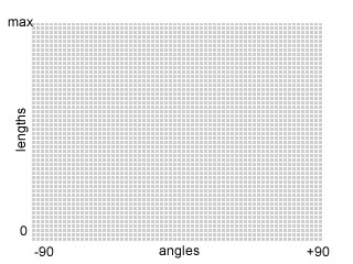
In this representation, a line is formed using two parameters - an angle θ and a distance p. p is the length of the normal from the origin (0, 0) onto the line. and θ is the angle this normal makes with the x axis. This solves the flaw perfectly.

The angle θ can be only from -90o to +90o and the length p can range from 0 to length of diagonal of the image. These values are finite, and thus you can "store" them on a computer without much trouble.

In this representation, the equation of the line is:

where  is a point through which the line passes.

With this new equation, we have a few changes in the end-point to line "transition" from the xy space to the pθ space. A line in the xy space is still equivalent to a point in the pθ space. But a point in the xy space is now equivalent to a sinusoidal curve in the pθ space.

The image at the top of this article is an actual pθ space. The sinusoidal curves have been generated while trying to figure out lines an image.

Implementation

With those ideas through, we're ready to implement the Hough transform. The idea is to let each pixel "vote". So an array of accumulator cells is created.

In our case, the accumulator cells form a 2D array. The horizontal axis is for the different θ values and the vertical axis for p values.

The accumulator

Next, you loop through every pixel of the edge detected image (Hough works only on edge detected images... not on normal images).

If a pixel is zero, you ignore it. It's not an edge, so it can't be a line. So move on to the next pixel.

If a pixel is nonzero, you generate its sinusoidal curve (in the pθ space). That is, you take θ = -90 and calculate the corresponding p value. Then you "vote" in the accumulator cell (θ, p). That is, you increase the value of this cell by 1. Then you take the next θ value and calculate the next p value. And so on till θ = +90. And for every such calculation, making sure they "vote".

So for every nonzero pixel, you'll get a sinusoidal curve in the pθ space (the accumulator cells). And you'll end up with an image similar to the one at the top.

Detecting lines

The image at the top has several "bright spots". A lot of points "voted" for this spot. And these are the parameters that describe the lines in the original image. Simple as that.

Accuracy

The accuracy of the Hough transform depends on the number of accumulator cells you have. Say you have only -900, -450, 00, 450 and 900 as the cells for θ values. The "voting" process would be terribly inaccurate. Similarly for the p axis. The more cells you have along a particular axis, the more accurate the transform would be.

Also, the technique depends on several "votes" being cast into a small region. Only then would you get those bright spots. Otherwise, differentiating between a line and background noise is one really tough job.

Done

Now you know how the standard Hough transform works! You can try implementing it... should be simple enough.

from: http://aishack.in/tutorials/hough-transform-normal/