Has your conversion rate changed? An introduction to Bayesian timeseries analysis with Python.
来源:互联网 发布:优绘下载 mac版 编辑:程序博客网 时间:2024/05/01 18:51
Has your conversion rate changed? An introduction to Bayesian timeseries analysis with Python.
When running a large site, it's important to monitor site behavior. For an ecommerce or similar site, the key thing to measure is conversion rate - if your conversion rate goes down, something is wrong. A common - but wrong - way to measure conversion rate is to simply use a rolling window. If the desired conversion rate is 5%, one might plot the conversion rate over the past 1 hour and trigger an alert if the conversion rate drops below some threshold.
Unfortunately, as Willie Wheeler observes in his blog post Monitoring Bookings and the Law of Large Numbers, a static threshold simply doesn't work. The problem is that variation in the number of visitors over time changes and a reduced number of visitors will increase the variance of your conversion rate. Consider the following scenario - a uniform 5% conversion rate. During some time periods the number of visitors is 10,000, while during others it's only 1,000.
Supose we were to raise an alert whenever the empirical conversion rate dropped below 4%. In this case, the false positive rate during periods when there are 10,000 visitors would be only binom(10000, 0.05).cdf(400) == 1.21e-06. That's pretty good! However, during the low traffic periods, that false positive rate rises to binom(1000, 0.05).cdf(40) = 0.081. Whoops!
In pictures, here's what happens:
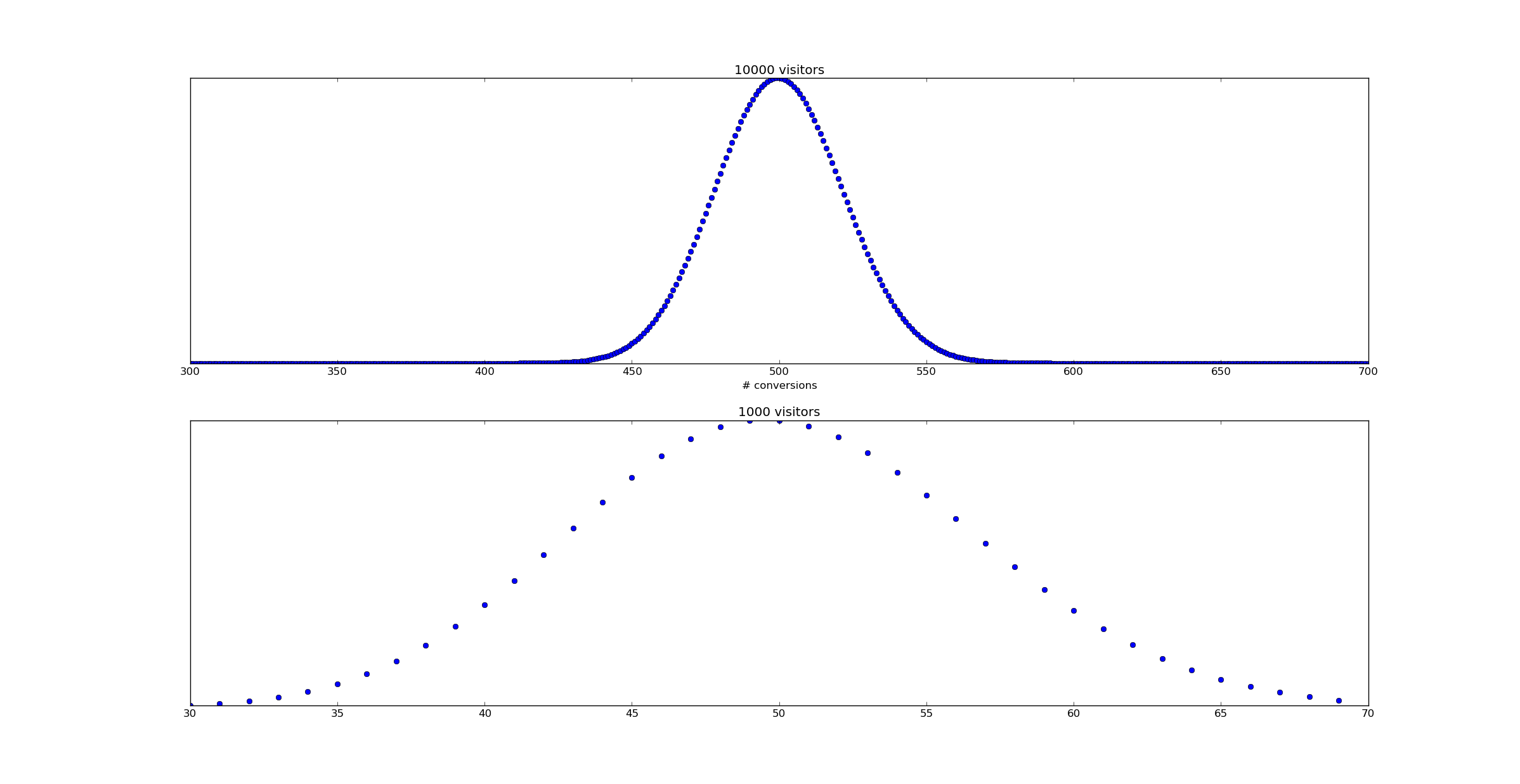
Based on this analysis it's pretty clear no static threshold can be used - a tight threshold for the 10,000 visitor time periods would have a huge number of false positives for the 1,000 visitor case.
This problem can be resolved by a Bayesian timeseries model.
Bayesian Timeseries Analysis
A timeseries is simply a function of time -
Here's the basic idea. Let us allow
So in simple terms:
If we could measure
But when the number of data points we have is lower - say 1,000 per unit time - it's harder to observe a jump.
How can we extract the maximal amount of information from the data available?
Computing the likelihood of a timeseries
Consider a timeseries
The likelihood is defined as
Now given a data series - a sequence of points
Sometimes more usefully, we might wish to consider the log likelihood:
Computing the likelihood with Python
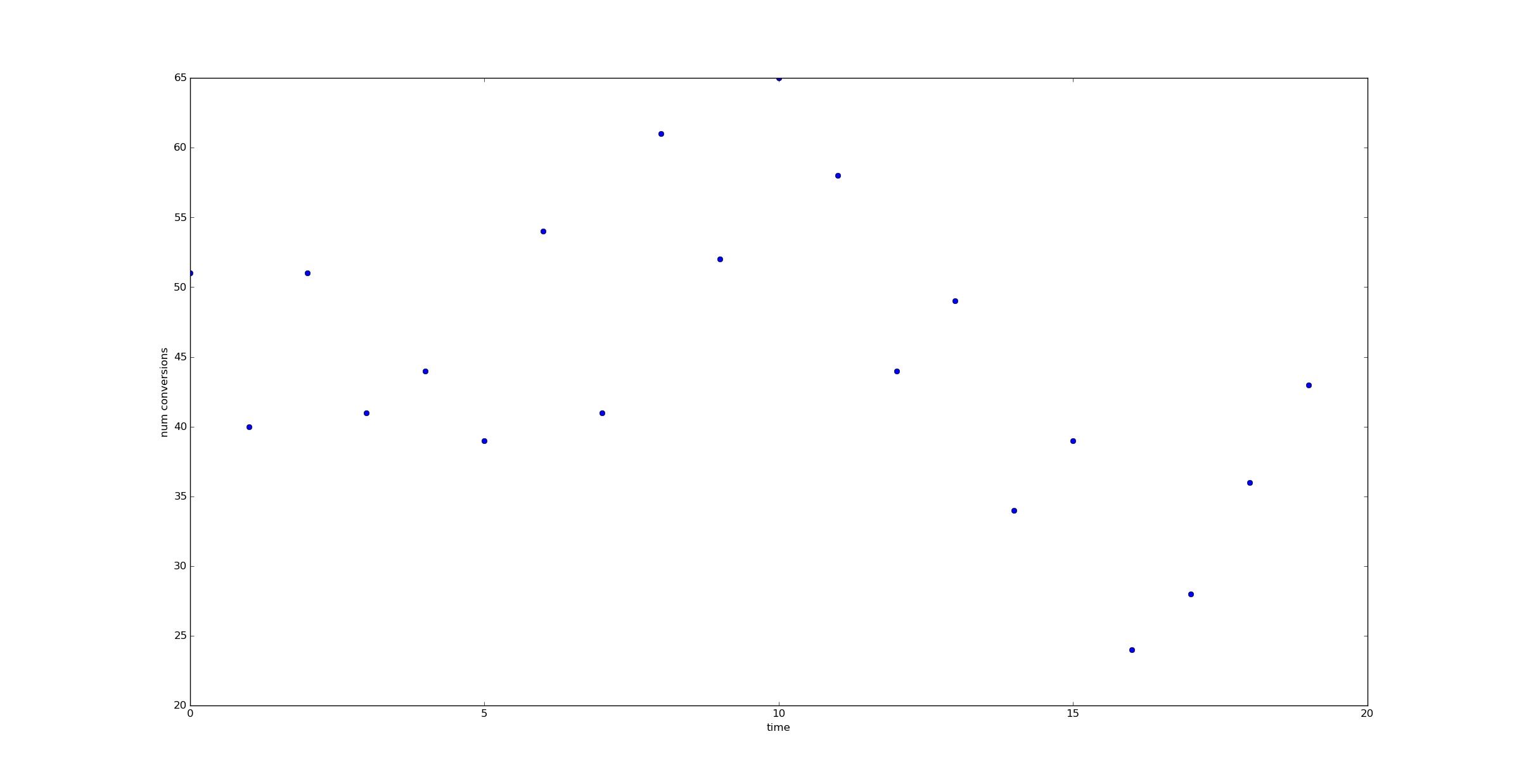
Suppose now we have input data - a timeseries n and c representing visitor count and conversions:
n = array([ 1000., 1000., 1000., 1000., 1000., 1000., 1000., 1000., 1000., 1000., 1000., 1000., 1000., 1000., 1000., 1000., 1000., 1000., 1000., 1000.])c = array([51, 40, 51, 41, 44, 39, 54, 41, 61, 52, 65, 58, 44, 49, 34, 39, 24, 28, 36, 43])Then let us represent theta with an array as well.
theta = array([ 0.05, 0.05, 0.05, 0.05, 0.05, 0.05, 0.05, 0.05, 0.05, 0.05, 0.05, 0.05, 0.05, 0.05, 0.05, 0.05, 0.05, 0.05, 0.05, 0.05])The log likelihood can be computed via:
def log_likelihood(n, c, theta): return sum(binom.logpmf(c, n, theta))And of course the likelihood itself can be computed via:
def likelihood(n, c, theta): return exp(log_likelihood(n,c,theta))Comparing likelihoods
Now let us imagine we had two alternate theories about what
Now consider an "alternate hypothesis" - the assumption that the conversion rate dropped from 5% to 3% at time 14.
This is a very specific alternate hypothesis (it's exactly how I generated the data) which I'm choosing for illustrative purposes. I put "null hypothesis" and "alternate hypothesis" in scare quotes since I'm not planning on using them in a Frequentist manner.
Using the likelihood formula for
and
(I've shifted to a log scale to make the numbers easier to observe.)
Now lets consider a range of alternate hypothesis, each representing the possibility of a jump at a different time:
We can plot the log likelihood of these various alternate hypothesis. The green line in this plot represents the "null hypothesis" that no jump occurred, and the conversion rate remained 5% for all time.
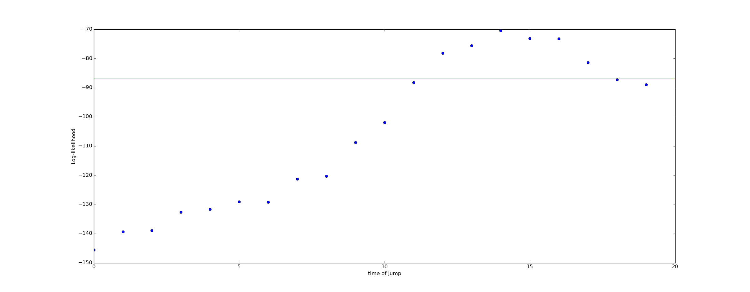
The fact that the log likelihood peaks at
Bayesian Inference
Bayesian inference takes our rough intuition - that we should consider a drop in conversion rate at
To do Bayesian inference, we need to come up with a prior. As a prior, I'll assume that a drop in conversion rate is unlikely - only 2%. I'll also assume that the probability of a drop occurring at any given time is equal.
For simplicity I'll assume that if a drop occurs, the drop is from 5% to 3%.
Thus, as a prior, we obtain:
To compute a posterior, we need to use Bayes rule:
So for example, we can compute the probability of there being no jump as:
In contrast, the probability of a jump at t=14 is:
Repeating this calculation for all times yields the following plot of the posterior on the time at which the conversion rate dropped:
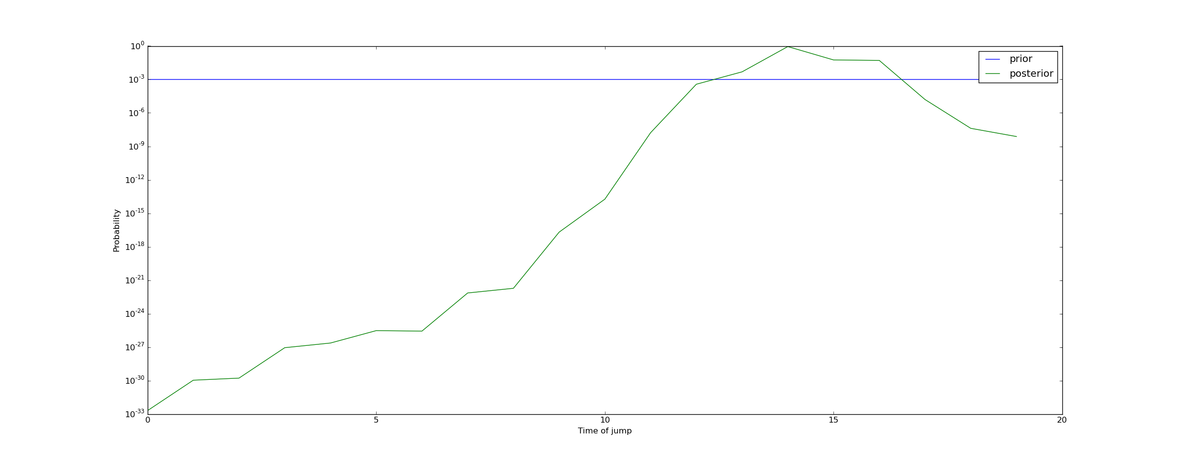
We can draw the conclusion that a jump almost certainly occurred (with probability 99.95%) at some point between t=13 and t=17. This means we should raise an alert!
Doing the calculation in Python
The following code implements the computation of the posterior:
from pylab import *from scipy.stats import binomdef log_likelihood(n, c, theta): return sum(binom.logpmf(c, n, theta))def bayesian_jump_detector(n, c, base_cr=0.05, null_prior=0.98, post_jump_cr=0.03): """ Returns a posterior describing our beliefs on the probability of a jump, and if so when it occurred. First return value is probability null hypothesis is true, second return value is array representing the probability of a jump at each time. """ theta = full(n.shape, base_cr) likelihood = zeros(shape=(n.shape[0] + 1,), dtype=float) #First element represents the probability of no jump likelihood[0] = null_prior #Set likelihood equal to prior likelihood[1:] = (1.0-null_prior) / n.shape[0] #Remainder represents probability of a jump at a fixed increment likelihood[0] = likelihood[0] * exp(log_likelihood(n, c, theta)) for i in range(n.shape[0]): theta[:] = base_cr theta[i:] = post_jump_cr likelihood[i+1] = likelihood[i+1] * exp(log_likelihood(n, c, theta)) likelihood /= sum(likelihood) return (likelihood[0], likelihood[1:])Experiments with other scenarios
If we now consider a situation with only 100 visitors/time unit, we can run this code as well.
n = full((20,), 100)c = binom(100, 0.05).rvs(20) #No jump in CR occursbayesian_jump_detector(n, c, null_prior=0.99)#Result is:(0.99888216914806816, array([ 7.28189038e-11, 2.20197564e-10, 6.65856870e-10, 2.40083185e-10, 4.26612169e-10, 1.29003536e-09, 7.91551819e-10, 1.40653598e-09, 7.23795867e-09, 6.33837938e-08, 1.91666673e-07, 1.17604609e-07, 1.22800167e-07, 3.71336237e-07, 3.87741199e-07, 6.88990834e-07, 3.54550985e-06, 1.82450034e-05, 2.71896088e-04, 8.22188376e-04]))In this case, our confidence in the null hypothesis has increased from 99% to 99.89%.
What if we put a jump in?
n = full((20,), 100)c = binom(100, 0.05).rvs(20)c[13:] = binom(100, 0.03).rvs(7) #Jump occurs at t=13bayesian_jump_detector(n, c, null_prior=0.99)#Result is:(0.92236200077388664, array([ 2.78977290e-06, 2.91302001e-06, 5.17624665e-06, 2.66366875e-05, 1.37070964e-04, 8.41052693e-05, 8.78208876e-05, 2.65562162e-04, 9.57518240e-05, 9.99819660e-05, 1.04398988e-04, 5.37231589e-04, 4.70461049e-03, 4.11989173e-02, 1.48547950e-02, 9.11474243e-03, 1.93120502e-03, 2.01652216e-03, 2.10560845e-03, 2.62158967e-04]))Because in this case we have a lot less data (100 data points/time unit vs 1000), we do not have as much confidence in our result. Our belief in the null hypothesis has dropped from 99% to 92%, and our belief that a drop has occurred near t=13 has increased to about 6% (with the remaining 2% spread out a little further). That's enough to raise an alert, but not enough to conclusively determine that the effect is real.
Conclusion
Bayesian timeseries analysis is just ordinary Bayesian statistics, but we are doing our analysis in a space of functions. Our goal is to characterize probabilistically an unknown function
In particular, I hope in a later post to comment on time varying conversion rates. Specifically, in another post on his blog, Willie Wheelerdiscusses the issue of time periodic conversion rates. I.e., the assumption here is that absent a negative downward spike,
- Has your conversion rate changed? An introduction to Bayesian timeseries analysis with Python.
- An Introduction to Machine Learning with Python
- An Introduction to Function Point Analysis
- An Introduction to Python Lists
- An Introduction to Python Lists
- warning C4996: 'swprintf': swprintf has been changed to conform with the ISO C standard, adding an e
- An Introduction to Network Programming with Java
- Video Introduction to Bayesian Data Analysis, Part 1: What is Bayes?
- Topic 3:An Informal Introduction to Python
- An Introduction to Interactive Programming in Python
- Introduction to Concurrent Programming with Stackless Python
- Introduction.to.Machine.Learning.with.Python 笔记
- JavaTech, an Introduction to Scientific and Technical Computing with Java
- An Introduction to Testing Web Applications with twill and Selenium
- An Essential Introduction to Maya Character Rigging with DVD
- An introduction to machine learning with scikit-learn
- An introduction to machine learning with scikit-learn
- An introduction to machine learning with scikit-learn
- 求x的n次方
- linux下查看已经安装的jdk 并卸载jdk
- <C#入门经典>学习笔记3之类型转换与枚举
- bzoj 4459: [Jsoi2013]丢番图 数学
- 快速排序(qsort)
- Has your conversion rate changed? An introduction to Bayesian timeseries analysis with Python.
- 输入成绩查看等级
- 各种优化方法总结比较(sgd/momentum/Nesterov/adagrad/adadelta)
- 设计模式C++策略模式
- 关于nginx 403问题
- js设置cookie,为cookie中设置多个key value
- 绝对定位的div居中
- 免费的优质英文字体打包下载
- 算法 - Dijkstra 最短路径