Rough Set Theory
来源:互联网 发布:java编写一个日历程序 编辑:程序博客网 时间:2024/05/22 12:41
开始从事数据挖掘方面的工作也已经有一年了,经常看CSND和国外一些博客上面的文章,但是从来也没有自己总结过,感觉很快就会忘记了,所以想从现在开始,用博客的方式来总结自己工作中的所学所得。
这篇关于Rough Set的整理主要是wiki上面的内容,因为找了好几个讲解Rough Set的资料感觉都不是很清晰,看到wiki上面的内容到时清楚明白,所以打算根据wiki上面的内容总结一下。
原文链接:点击打开链接 (https://en.wikipedia.org/wiki/Rough_set)
1. Definitions
1.1 Information system framework
Let  be an information system (attribute-value system).
 is a non-empty set of finite objects (the universe) = {
 ~
~  }
}
 is a non-empty, finite set of attributes = {
 ~
~  }
}
Such that  for every
  .
.
 is the set of values that attribute
  may take. = {0, 1, 2} if =
 is the value of object
  's attribute 's value. = 1 if = and =
An example of Information system table:

With any  there is an associated equivalence relation
  :
:

The relation is called a  -indiscernibility relation.
The partition of is a family of all equivalence classes of and is denoted by  (or
(or  ).
).
If 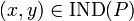 , then and
  are indiscernible (or indistinguishable) by attributes from .
For example:
if 
so the equivalence classes:

if attribute  alone is selected
so the equivalence classes:

1.2 Definition of a Rough Set
Let  be a target set that we wish to represent using attribute subset .
For example
consider the target set 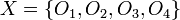 , and let attribute subset , the full available set of features. It will be noted that the set
  cannot be expressed exactly, because in
 ![[x]_P,](https://upload.wikimedia.org/math/4/b/2/4b2ce85c6c6b6e44983871c5a57b580b.png) , objects
, objects  are indiscernible. Thus, there is no way to represent any set which includes
  but excludes objects
  and .
and .
However, the target set can be approximated using only the information contained within by constructing the -lower and -upper approximations of :
![{\underline P}X= \{x \mid [x]_P \subseteq X\}](https://upload.wikimedia.org/math/e/4/f/e4f4ec93ab81c92a337b3aa636e65e54.png)
![{\overline P}X = \{x \mid [x]_P \cap X \neq \emptyset \}](https://upload.wikimedia.org/math/b/8/8/b88264ed716b07d8885f3ddef897e54a.png)
Lower approximation and positive region

![[x]_P](https://upload.wikimedia.org/math/5/7/1/5716347ab104065a9ec16d77ec9c6b62.png) which are contained by (i.e., are subsets of) the target set. that can be positively (i.e., unambiguously) classified as belonging to target set .
which are contained by (i.e., are subsets of) the target set. that can be positively (i.e., unambiguously) classified as belonging to target set .Upper approximation and negative region
 which have non-empty intersection with the target set.
The upper approximation is the complete set of objects that in that cannot be positively (i.e., unambiguously) classified as belonging to the complement ( ) of the target set . In other words, the upper approximation is the complete set of objects that are possibly members of the target set . The set
  therefore represents the negative region, containing the set of objects that can be definitely ruled out as members of the target set.
Boundary region
The boundary region, given by set difference  , consists of those objects that can neither be ruled in nor ruled out as members of the target set .
The rough set
The tuple  composed of the lower and upper approximation is called a rough set; thus, a rough set is composed of two crisp sets, one representing a lower boundary of the target set , and the other representing an upper boundary of the target set .
The accuracy of the rough-set representation of the set :

,  ,
,  , is the ratio of the number of objects which can positively be placed in to the number of objects that can possibly be placed in – this provides a measure of how closely the rough set is approximating the target set.
1.3 Definability
if  , we say the is definable on attribute set , otherwise, it's undefinable.
is internally undefinable if  and
and  . This means that on attribute set , there are objects which we can be certain belong to target set , but there are no objects which we can definitively exclude from set . is externally undefinable if
  and
and  . This means that on attribute set , there are no objects which we can be certain belong to target set , but there are objects which we can definitively exclude from set . is totally undefinable if and . This means that on attribute set , there are no objects which we can be certain belong to target set , and there are no objects which we can definitively exclude from set . Thus, on attribute set , we cannot decide whether any object is, or is not, a member of .
1.4 Reduct and core
Formally, a reduct is a subset of attributes  such that
![[x]_{\mathrm{RED}}](https://upload.wikimedia.org/math/7/3/e/73eaf34c3ce3fa25f830b13b74825f93.png) = , that is, the equivalence classes induced by the reduced attribute set
= , that is, the equivalence classes induced by the reduced attribute set  are the same as the equivalence class structure induced by the full attribute set .
- the attribute set is minimal, in the sense that
![[x]_{(\mathrm{RED}-\{a\})} \neq [x]_P](https://upload.wikimedia.org/math/2/d/f/2dfaba469477c41fa58ad8eab9b45308.png) for any attribute
for any attribute  ; in other words, no attribute can be removed from set without changing the equivalence classes .
attribute set
 is a reduct, and the equivalence class structure is
and same with the .So we can say the former one is a reduct of the latter one. Moreover, the reduct is not unique and for this instance,  is also a reduct for the .
The set of attributes which is common to all reducts is called the core
for the two reducts and , the common attribute is ,which is the core of equivalence-class structure. If is drop out of the attribute set, the equivalence-class structure will be changed.
Note that it is possible for the core to be empty, whicn means that there is no indispensable attribute:any single attribute in such an information system can be deleted without altering the equivalence-class structure. In such cases, there is no essential or necessary attribute which is required for the class structure to be represented.
后面还有Attribute dependency, Rule extraction, Incomplete data三部分,待以后再看。
————————————————————————————————————————————————————————————————————————————————————————————————————————————————————————————————————
时隔多日,终于又可以开始搞自己的小研究了,最近读了一篇Rough set 和 DS evidence 相结合文章,其中利用Rough set做权值计算,在这里整理一下:
基本定义:
在这里由于文献中使用的公式与wiki里的稍有不同,我们重新定义一下:
定义一个信息系统:
其中,
是一个非空的对象集,也就是说上面的O1, O2,...
是条件属性集,一共有m个条件属性(Condition Attribute)
是决定属性集,一共有n个决定属性(Decision Attribute),但通常我们只有一个
则对于所有条件属性C的等价关系定义为:
该定义表示为:两个主体对象x,y,如果对于条件属性C中的所有条件属性,他们两个的值都相等,那么x,y就是等价的(也就是说不可分的indiscernible)
同样的,对于去除了Cj之后(即从条件属性集C中去除第j个条件属性)的等价关系定义为:
该定义表示,不考虑第j个条件属性,如果x,y两个主体对象所有其他的条件属性都对应相等,那么他们就是等价的或者说是不可分的
对于决定属性D,同样也有等价关系,定义为:
该定义也挺简单,就是根据决定属性,只要是所有对应的决定属性的值相等,那么两个主体对象x,y就是等价的
根据上面的等价条件公式,我们可以得到针对不同条件下的知识系统(Knowledge system)
主体对象们 U 对于条件属性全集 C 的知识系统,等价于上文中的
的
为主体对象U对于去除了第j个条件属性后的知识系统,
为主体对象U对于决定属性的知识系统
权值计算:
针对上面的基本定义,下面来计算各个属性的权值(weight,对于决定书信的重要性):
Definition 1:决定属性 D 对于条件属性全集 C 的依赖度

Definition 2:第 j个条件属性的显著性(significance)的计算

Definition 3:计算权值(归一化)

同样的,举个“栗子”:
OK,根据表里的数据我们开始计算每个专家做出的预测的权重是多少啦。
1. 首先,根据基本概念,我们要计算出要用的各个等价关系和知识系统。

根据我们计算权重的原理(熵理论),我们要首先计算出在有所有专家都参与的系统中的熵是多少,根据Definition 1,我们可以计算得到:

根据Definition 2,我们可以计算得到:


这里需要注意的一点是关于计算公式中 0×ln0 的值的问题,在信息熵(Information Entropy)理论中,0×ln0的值为0。可以参考wiki,传送门:点击打开链接这里贴上这段话:

根据Definition 3,我们可以得到:

通过以上的计算过程,我们可以得到:
Expert 1在决策时的权重为1,而Expert 2和Expert 3的决策权重均为零(也就是说Expert 1说的靠谱,而Expert 2 和 3都不靠谱(相比较Expert 1而言))。
OK, that's all.
Thanks for your watching!
- Rough Set Theory
- 粗糙集(Rough set) 理论
- 粗糙集(Rough Set)约简系统软件
- 粗糙集(Rough Set)约简系统软件
- 粗糙集(Rough Set)约简系统软件
- Rough set的rule提取LEM2算法
- Tutorial on Axiomatic Set Theory
- game theory课程week2 problem set
- game theory week1 problem set 1
- UVa10356 - Rough Roads(Dijkstra)
- database rough 1
- UVa 193 - Graph Coloring(graph theory, brute force, backtracking, NP-complete, maximum independent set.)
- VMware architecture - a rough picture
- Rough Draft Ad Analysis Paper
- Graph Theory
- Probability Theory
- pcr theory
- tomcat theory
- 使用CD-K算法实现RBM
- Linux下创建库函数
- Leetcode 139. Word Break & 140. Word Break II
- 【设计模式】正确使用单例模式
- linux基础之常用命令(1)
- Rough Set Theory
- linux boa服务器配置解析
- OSI 参考模型与TCP/IP 参考模型的比较
- adb logcat调试中常用的命令介绍
- 非常经典的JAVA编程题(水仙花数)
- listview更改数据
- 区块链网络动力学对世界的解构和重构
- 驱动中获取进程名的正确方法
- java 代码