Ordered dithering

From Wikipedia, the free encyclopedia

In this example image (Lenna), the photograph shown on left has been quantizedto 16 colors and dithered using the 8x8 ordered dithering pattern.

The characteristic 15 patterns of the 4x4 ordered dithering matrix - seen clearly when used with only two colors, black and white, on top of its undithered original

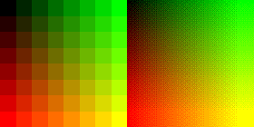
Ordered dithering is an image dithering algorithm. It is commonly used by programs that need to provide continuous image of higher colors on a display of less color depth. For example, Microsoft Windows uses it in 16-color graphics modes. It is easily distinguished by its noticeable crosshatch patterns.

The algorithm achieves dithering by applying a threshold map on the pixels displayed, causing some of the pixels to be rendered at a different color, depending on how far in between the color is of available color entries.

Different sizes of threshold maps exist:

{\displaystyle {\frac {\displaystyle 1}{\displaystyle 5}}{\begin{bmatrix}1&3\\4&2\\\end{bmatrix}}}

{\displaystyle {\frac {\displaystyle 1}{\displaystyle 10}}{\begin{bmatrix}1&8&4\\7&6&3\\5&2&9\\\end{bmatrix}}}

{\displaystyle {\frac {\displaystyle 1}{\displaystyle 17}}{\begin{bmatrix}1&9&3&11\\13&5&15&7\\4&12&2&10\\16&8&14&6\\\end{bmatrix}}}

{\displaystyle {\frac {\displaystyle 1}{\displaystyle 65}}{\begin{bmatrix}1&49&13&61&4&52&16&64\\33&17&45&29&36&20&48&32\\9&57&5&53&12&60&8&56\\41&25&37&21&44&28&40&24\\3&51&15&63&2&50&14&62\\35&19&47&31&34&18&46&30\\11&59&7&55&10&58&6&54\\43&27&39&23&42&26&38&22\\\end{bmatrix}}}

The map may be rotated or mirrored without affecting the power of the algorithm. This threshold map (for sides with length as power of two) is also known as anindex matrix or Bayer matrix.^[1]

Arbitrary size threshold maps can be devised with a simple rule: First fill each slot with a successive integer starting from 1. Then reorder them such that the average distance between two successive numbers in the map is as large as possible, ensuring that the table "wraps" around at edges.^{[citation needed]}

The algorithm renders the image normally, but for each pixel, it adds a value from the threshold map, causing the pixel's value to be quantized one step higher if it exceeds the threshold. For example, in monochrome rendering, if the value of the pixel (scaled into the 0-9 range if using a 3x3 matrix) is less than the number in the corresponding cell of the matrix, plot that pixel black, otherwise, plot it white.

A color scale shown undithered and dithered. The palette has 8 red tones, 8 green tones, and their intersections for a total of 64 colors, whereas the original image has 140 in both directions for a total of 19600 colors.

In pseudocode:

 foreach y    foreach x       oldpixel := pixel[x][y] + (pixel[x][y] * threshold_map_4x4[x mod 4][y mod 4])       newpixel := find_closest_palette_color(oldpixel)       pixel[x][y] := newpixel

The values read from the threshold map should scale into the same range as is the minimal difference between distinct colors in the target palette.

Because the algorithm operates on single pixels and has no conditional statements, it is very fast and suitable for real-time transformations. Additionally, because the location of the dithering patterns stays always the same relative to the display frame, it is less prone to jitter than error-diffusion methods, making it suitable for animations. Because the patterns are more repetitive than error-diffusion method, an image with ordered dithering compresses better. Ordered dithering is more suitable for line-art graphics as it will result in straighter lines and fewer anomalies.

The size of the map selected should be equal to or larger than the ratio of source colors to target colors. For example, when quantizing a 24bpp image to 15bpp (256 colors per channel to 32 colors per channel), the smallest map one would choose would be 4x2, for the ratio of 8 (256:32). This allows expressing each distinct tone of the input with different dithering patterns.^{[citation needed]}

Notes[edit]

1. Jump up^ Bayer, Bryce (June 11–13, 1973). "An optimum method for two-level rendition of continuous-tone pictures" (PDF). IEEE International Conference on Communications 1: 11–15.

References[edit]

• Ordered Dithering (Graphics course project, Visgraf lab, Brazil)
• Dithering algorithms (Lee Daniel Crocker, Paul Boulay and Mike Morra)
• Arbitrary-palette positional dithering algorithm (Joel Yliluoma)