信号处理——Hilbert端点效应浅析

作者：桂。

时间：2017-03-05  19:29:12

链接：http://www.cnblogs.com/xingshansi/p/6506405.html 

声明：转载请注明出处，谢谢。

---

 

 

前言

本文为Hilbert变换分析的补充，主要介绍Hilbert变换中的端点效应，内容拟分两部分展开：

　　1）Gibbs现象介绍；

　　2）端点效应分析；

内容为自己一家之言，其中不合理的地方，希望各位告诉我，反正改不改是我的事(●'◡'●)

 

 

 

 

 

一、Gibbs现象

 关于Gibbs的理论推导，可以参考郑君里的《信号与系统》上册（第二版，P97~101），里边有详细的理论分析。也可参考：维基百科，里边有一张图很形象：

给出对应的代码（用该程序，借助MATLAB便可以生成.gif图）：

%% 代码介绍========================================================================%% Title: %  1) Fourier series approximation of square wave.%  2) Demonstration of Gibbs phenomenon (verification of Fig. 3.9 of [1])%% Author: %  Ankit A. Bhurane ([e-mail])%% Expression:% The Fourier series approximation of a square wave signal existing between% -Tau/2 to Tau/2 and period of T0 will have the form:%% Original signal to be approximated: %                         :%               __________:__________  A%              |          :          |%              |          :          |%              |          :          |%    __________|          :          |__________% -T0/2     -Tau/2        0        Tau/2       T0/2%                         :%                         :%% Its Fourier series approximation:%%                  Inf   %                  ___ %         A*Tau   \     / sin(pi*n*Tau/T0)                    \% r(t) = -------   |   | ------------------ exp^(j*n*2*pi/T0*t) |%          T0     /___  \  (pi*n*Tau/T0)                      /%               n = -Inf %% The left term inside summation are the Fourier series coeffs (Cn). The% right term is the Fourier series kernel. % Tau: range of square wave, T: period of the square wave, % t: time variable, n: number of retained coefficients.% %% Observations:% 1) As number of retained coefficients tends to infinity, the approximated% signal value at the discontinuity converge to half the sum of values on% either side. % 2) Ripples does not decrease with increasing coefficients with% approximately 9% overshoot.% 3) Energy in the error between original and approximated signal, reduces% as the number of retained coefficients are increased.% %% References: % [1] Oppenheim, Willsky, Nawab, "Signals and Systems", PHI, Second edition% [2] Dean K. Frederick and A. Bruce Carlson, "Fourier series" section in %     Linear systems in communication and control %% Last Modified: Sept 24, 2013.%% Copyright (c) 2013-2014 | Ankit A. Bhurane%% 

　　

clc; clear all; close all;% SpecificationA = 1; % Peak-to-peak amplitude of square waveTau = 10; % Total range in which the square wave is defined (here -5 to 5)T0 = 20; % Period (time of repeatation of square wave), here 10 C = 200; % Coefficients (sinusoids) to retain N = 1001; % Number of points to considert = linspace(-(T0-Tau),(T0-Tau),N); % Time axisX = zeros(1,N); X(t>=-Tau/2 & t<=Tau/2) = A; % Original signalR = 0; % Initialize the approximated signalk = -C:C; % Fourier coefficient number axisf = zeros(1,2*C+1); % Fourier coefficient values% Loop for plotting approximated signals for different retained coeffs.for c = 0:C % Number of retained coefficients    for n = -c:c % Summation range (See equation above in comments)                % Sinc part of the Fourier coefficients calculated separately         if n~=0            Sinc = (sin(pi*n*Tau/T0)/((pi*n*Tau/T0))); % At n NOTEQUAL to 0        else            Sinc = 1; % At n EQUAL to 0        end        Cn = (A*Tau/T0)*Sinc; % Actual Fourier series coefficients        f(k==n) = Cn; % Put the Fourier coefficients at respective places        R = R + Cn*exp(1j*n*2*pi/T0.*t); % Sum all the coefficients    end        R = real(R); % So as to get rid of 0.000000000i (imaginary) factor    Max = max(R); Min = min(R); M = max(abs(Max),abs(Min)); % Maximum error    Overshoot = ((M-A)/A)*100; % Overshoot calculation    E = sum((X-R).^2); % Error energy calculation        % Plots:    % Plot the Fourier coefficients    subplot 211; stem(k,f,'m','LineWidth',1); axis tight; grid on;    xlabel('Fourier coefficient index');ylabel('Magnitude');    title('Fourier coefficients');        % Plot the approximated signal    subplot 212; plot(t,X,t,R,'m','LineWidth',1); axis tight; grid on;     xlabel('Time (t)'); ylabel('Amplitude');    title(['Approximation for N = ', num2str(c),...    '. Overshoot = ',num2str(Overshoot),'%','. Error energy: ',num2str(E)])    pause(0.1); % Pause for a while    R = 0; % Reset the approximation to calculate new oneend

　　简而言之：

• 对于跳变的点，傅里叶变换的分量只能是能量收敛，而不是一致（幅度）收敛；
• 对于跳变的点，如门函数/方波，信号由低频到高频众多分量组合而成。

故对于连续时域信号，Fourier级数只能无限项逼近，不能完全一致。 

 

二、端点效应

　　A-理论解释

借用之前博文的一张图：

连续信号到离散信号需要进行采样，由于有无穷多项，采样率对于高频的部分（因为无穷多项）难以满足Nyquist采样定理，因此会出现失真，这也就是端点效应的理论解释。失真的根本原因在时域采样，频域采样步骤只不过影响频域分辨率，即所谓的栅栏效应，但不是造成失真的根本原因。

　　B-现象分析

为了验证理论，此处采样一个正弦信号进行分析，按连续信号来看其Hilbert变换应该是余弦信号。

给出代码：

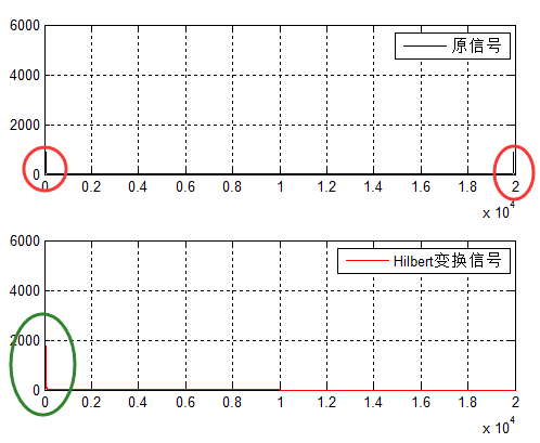
clc;clear all;close all;fs = 2000;f0 = 80;t = 0:1/fs:.1;sig = sin(2*pi*f0*t);sig_ref = -cos(2*pi*f0*t);sig_hilbert = hilbert(sig);figure;subplot 311plot(t,sig,'k','linewidth',2);hold on;plot(t,sig_ref,'r.-','linewidth',2);hold on;plot(t,imag(sig_hilbert),'b','linewidth',2);hold on;legend('原信号','余弦信号','Hilbert变换信号','localization','best');ylim([-2,2]);grid on;%频谱f = linspace(0,fs,length(t));subplot 312plot(f,abs(fft(sig)),'k');hold on;plot(f,abs(fft(sig_hilbert)),'r');hold on;legend('原信号','Hilbert变换信号','localization','best');grid on;

　　对应的结果图：

时域：

可以看到明显的端点效应（说是端点效应，如果间断点在中间位置，一样会有该效应，毕竟都是Nyquist定理下的误差嘛）。

频域：

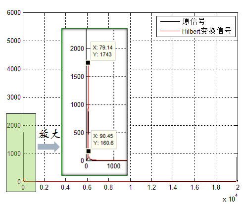
采样率取得够大了，理论上正弦信号Hilbert之后应该是一个单边的冲击。但频谱显示，峰值旁边的一个点，幅度达到160.6，这也印证了能量的泄露。

发现端点效应，与前文理论对应：Hilbert就是一个频域的变相器，本质也是fourier变换，是不是也因为跳变点（即信号中的Gibbs问题）？观察频谱，峰值旁边的点，幅值有160.5大小，我们计算原信号

2*sig(1)-sig(2)

　　得到结果是：-0.4820，而对于没有的点，应该是默认是0的，因此端点算是一个跳变点了。

注意：端点效应是相对于连续信号来讲，存在失真，从而出现误差。对于数字信号，Hilbert变换结果就是该正弦数字信号的精确表达，即逆Hilbert可以完全恢复出正弦信号。给一张Hilbert变换后，进行逆Hilbert变换的code及示意图：

clc;clear all;close all;fs = 2000;f0 = 40;t = 0:1/fs:.1;sig = sin(2*pi*f0*t);sig_hilbert = -imag(hilbert(imag(hilbert(sig))));figure;plot(t,sig,'k','linewidth',2);hold on;plot(t,sig_hilbert,'r--','linewidth',2);ylim([-2,2]);grid on;

　　从图中，可以看到从Hilbert结果恢复的信号与原信号完全一致！这也印证了上文的观点：失真在时域采样，而不在频域采样。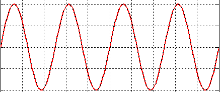

下面再做一组实验，验证推断：
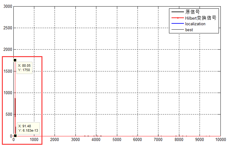
思路——只要保证2sig(1)-sig(2)逼近0，理论上是不是就没有边界效应了？
此时：2*sig(1)-sig(2)=1.5873e-05，再来看看结果图：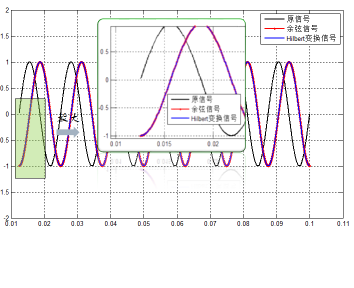

 再来看看频谱，没错，峰值旁边的点压的很小（6.183e-13），符合预期。

此处代码：

clc;clear all;close all;fs = 20000;f0 = 80;t = 0.01255:1/fs:.1;%t = 0.0252:1/fs:.1则没有跳变。sig = sin(2*pi*f0*t);2*sig(1)-sig(2)sig_ref = -cos(2*pi*f0*t);sig_hilbert = hilbert(sig);figure;subplot 211plot(t,sig,'k','linewidth',2);hold on;plot(t,sig_ref,'r.-','linewidth',2);hold on;plot(t,imag(sig_hilbert),'b','linewidth',2);hold on;legend('原信号','余弦信号','Hilbert变换信号','localization','best');ylim([-2,2]);grid on;%频谱f = linspace(0,fs,length(t));subplot 212plot(f,abs(fft(sig)),'k');hold on;plot(f,abs(fft(sig_hilbert)),'r');hold on;legend('原信号','Hilbert变换信号','localization','best');ylim([0 6000]);grid on;

基于这个基本要点，很多方法对信号：预测、延拓、镜像等操作，以消除或者降低端点效应。为什么用2*sig(1)-sig(2)呢，这是因为实验的函数为sin，在0附近sinx~x ，严格意义上应该是2*f(1)-f(2)≈ 0 。f是函数表达式，而且实际中信号不是单一频点，仅仅通过两个点判断也是不够的。
只是消除端点方法不同，但端点现象的本质一致。
多说一句：Hilbert将双边谱压成单边，这让频域滤波等操作方便了不少。

参考：

Gibbs phenomen:https://en.wikipedia.org/wiki/Gibbs_phenomenon