通过GBDT组合的特征作为LR的输入

来源：互联网发布：和平网络电视频道地址编辑：程序博客网时间：2024/04/30 18:03

scikit-learn中的apply() 函数有什么作用？

在最新版本的scikit-learn中，gradient boosting新增了apply()方法。如图：

请问，这个函数功能是和 facebook使用的 GBDT + LR 是类似的么？

如果类似，请问该怎么利用好这个函数？或者如何使得它的效果和facebook的方法一样？

作者：知乎用户
链接：https://www.zhihu.com/question/39254529/answer/80440989
来源：知乎
著作权归作者所有。商业转载请联系作者获得授权，非商业转载请注明出处。

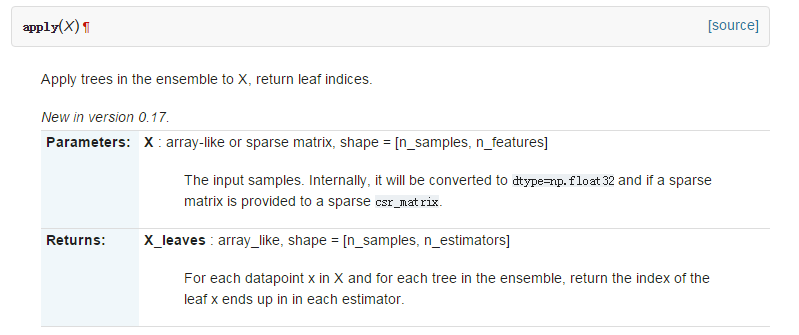
我觉得你看这个就可以了。Feature transformations with ensembles of trees
讲的已经很详细了，我的理解是，apply可以把特征转换到一个更高维空间形成稀疏矩阵，然后就可以用线性模型了。这个思想和SVM里的核函数有点类似。
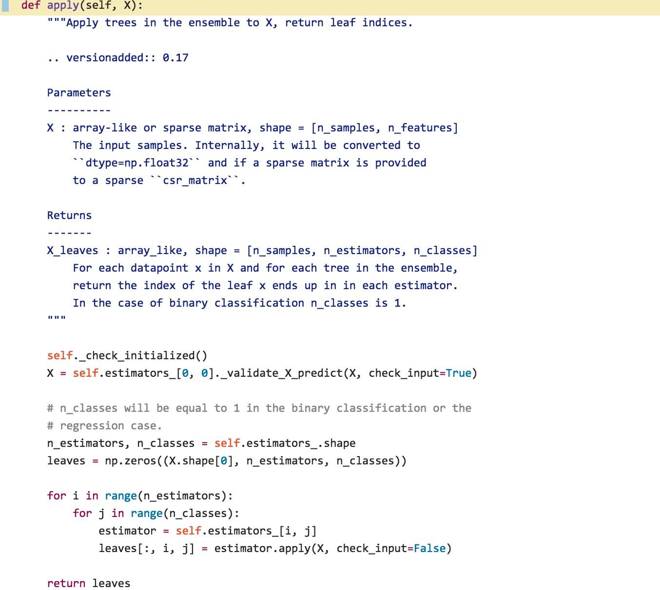
你看看它的代码：

至于这个函数怎么用，你看看它自带的例子，效果比一般的rf/gbdt要好。

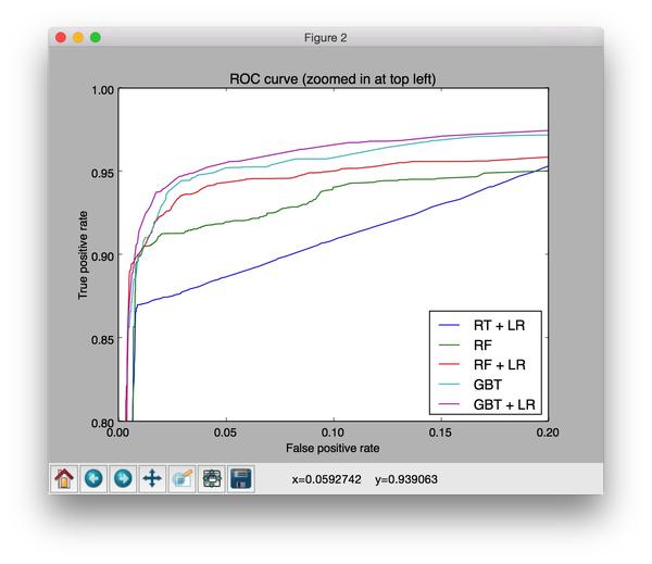
ROC曲线上来看，GBT+LR的效果是最好的。

我自己不用Python，不过推荐你用xgboost里xgboost.Booster的predict方法并将pred_leaf设置成TRUE，得到的结果应该是一样的，而且应该更好。因为xgboost自带一定的regularization而且利用了二阶泰勒展开的信息，所以学出来的feature应该会更好一些。因为Boosting本身就是一个学feature的过程，Friedman自己把Boosting过程看作是Additive Logistic Regression。其实得到的矩阵可以理解为很多Categorical Variable的不同Level，One-Hot Encoding展开了就是稀疏矩阵。
另外也要看你GBDT后面用什么模型，如果是Logistic Regression就One-Hot Encoding，如果后面是LibFFM，就直接用index，这样Variance应该还会小一些。

import numpy as npnp.random.seed(10)import matplotlib.pyplot as pltfrom sklearn.datasets import make_classificationfrom sklearn.linear_model import LogisticRegressionfrom sklearn.ensemble import (RandomTreesEmbedding, RandomForestClassifier,                              GradientBoostingClassifier)from sklearn.preprocessing import OneHotEncoderfrom sklearn.model_selection import train_test_splitfrom sklearn.metrics import roc_curvefrom sklearn.pipeline import make_pipelinen_estimator = 10X, y = make_classification(n_samples=80000)X_train, X_test, y_train, y_test = train_test_split(X, y, test_size=0.5)# It is important to train the ensemble of trees on a different subset# of the training data than the linear regression model to avoid# overfitting, in particular if the total number of leaves is# similar to the number of training samplesX_train, X_train_lr, y_train, y_train_lr = train_test_split(X_train,                                                            y_train,                                                            test_size=0.5)# Unsupervised transformation based on totally random treesrt = RandomTreesEmbedding(max_depth=3, n_estimators=n_estimator,    random_state=0)rt_lm = LogisticRegression()pipeline = make_pipeline(rt, rt_lm)pipeline.fit(X_train, y_train)y_pred_rt = pipeline.predict_proba(X_test)[:, 1]fpr_rt_lm, tpr_rt_lm, _ = roc_curve(y_test, y_pred_rt)# Supervised transformation based on random forestsrf = RandomForestClassifier(max_depth=3, n_estimators=n_estimator)rf_enc = OneHotEncoder()rf_lm = LogisticRegression()rf.fit(X_train, y_train)rf_enc.fit(rf.apply(X_train))rf_lm.fit(rf_enc.transform(rf.apply(X_train_lr)), y_train_lr)y_pred_rf_lm = rf_lm.predict_proba(rf_enc.transform(rf.apply(X_test)))[:, 1]fpr_rf_lm, tpr_rf_lm, _ = roc_curve(y_test, y_pred_rf_lm)grd = GradientBoostingClassifier(n_estimators=n_estimator)grd_enc = OneHotEncoder()grd_lm = LogisticRegression()grd.fit(X_train, y_train)grd_enc.fit(grd.apply(X_train)[:, :, 0])grd_lm.fit(grd_enc.transform(grd.apply(X_train_lr)[:, :, 0]), y_train_lr)y_pred_grd_lm = grd_lm.predict_proba(    grd_enc.transform(grd.apply(X_test)[:, :, 0]))[:, 1]fpr_grd_lm, tpr_grd_lm, _ = roc_curve(y_test, y_pred_grd_lm)# The gradient boosted model by itselfy_pred_grd = grd.predict_proba(X_test)[:, 1]fpr_grd, tpr_grd, _ = roc_curve(y_test, y_pred_grd)# The random forest model by itselfy_pred_rf = rf.predict_proba(X_test)[:, 1]fpr_rf, tpr_rf, _ = roc_curve(y_test, y_pred_rf)plt.figure(1)plt.plot([0, 1], [0, 1], 'k--')plt.plot(fpr_rt_lm, tpr_rt_lm, label='RT + LR')plt.plot(fpr_rf, tpr_rf, label='RF')plt.plot(fpr_rf_lm, tpr_rf_lm, label='RF + LR')plt.plot(fpr_grd, tpr_grd, label='GBT')plt.plot(fpr_grd_lm, tpr_grd_lm, label='GBT + LR')plt.xlabel('False positive rate')plt.ylabel('True positive rate')plt.title('ROC curve')plt.legend(loc='best')plt.show()plt.figure(2)plt.xlim(0, 0.2)plt.ylim(0.8, 1)plt.plot([0, 1], [0, 1], 'k--')plt.plot(fpr_rt_lm, tpr_rt_lm, label='RT + LR')plt.plot(fpr_rf, tpr_rf, label='RF')plt.plot(fpr_rf_lm, tpr_rf_lm, label='RF + LR')plt.plot(fpr_grd, tpr_grd, label='GBT')plt.plot(fpr_grd_lm, tpr_grd_lm, label='GBT + LR')plt.xlabel('False positive rate')plt.ylabel('True positive rate')plt.title('ROC curve (zoomed in at top left)')plt.legend(loc='best')plt.show()

0 0