梯度下降法的matlab实现

NOTE:这是本人在学习NG课程后，尝试练习的用matlab实现的梯度下降算法。具体的梯度下降法的知识点不在赘述。
请参考线性回归 梯度下降知识点
一、线性回归（Linear Regression）
方法一利用公式 :（懂了）

function [ theta ] = linearReg()%线性回归。X=[1 1;1 2;1 3;1 4];  %注意第一列全为1，即x0=1,第二列才为x1Y=[1.1;2.2;2.7;3.8];A=inv(X'*X);theta=A*X'*Y;   %根据公式theta=(X'*X)^(-1)*X'*Y;end

注释：
1.这种方法最简单，但是公式推导过程很复杂
2.inv() 求逆
3. X ’是求X的转置
方法二：使用梯度下降法迭代（代码不懂）

function theta=linearRegression()%   梯度下降法寻找最合适的theta，使得J最小options=optimset('GradObj','on','MaxIter',100);inittheta=[1 1]';theta=fminunc(@costFunc,inittheta,options);end%%function  [J,gradient]= costFunc(theta)%J为代价函数。%y=theta(0)*x0+theta(1)*x1; 找出最好的theta来拟合曲线。%使得J最小的theta就是最好的thetax=[1;2;3;4];y=[1.1;2.2;2.7;3.8];m=size(x,1);hypothesis=theta(1)+theta(2)*x;delta=hypothesis-y;J=sum(delta.^2)/(2*m);gradient(1)=sum(delta.*1)/m;  %x0=1;gradient(2)=sum(delta.*x)/m;end

注释：
1.Matlab中fminunc函数的意义 以及options函数的初级用法
2.
function theta=linearRegression()
% 梯度下降法寻找最合适的theta，使得J最小
options=optimset(‘GradObj’,’on’,’MaxIter’,100);
inittheta=[1 1]’;
theta=fminunc(@costFunc,inittheta,options);
end
结合注释1，这个目前看不懂，先记住，这是梯度下降算法的一个小套路吧！
3.这两种方法，都采用数据：

x=[1;2;3;4];
y=[1.1;2.2;2.7;3.8];

当然，用的时候可以换成其它数据，两种方法得出的结果都是

theta =    0.3000    0.8600

即可以学习到线性函数：
Y=0.3000+0.8600*X;
补充：
第一个代码计算梯度下降（懂了）

clear allclc% training sample data;p0=26;p1=73;x=1:3;y=p0+p1*x;num_sample=size(y,2);% gradient descending process% initial values of parameterstheta0=1;theta1=3;%learning ratealpha=0.08;% if alpha is too large, the final error will be much large.% if alpha is too small, the convergence will be slowepoch=500;for k=1:epoch   v_k=k   h_theta_x=theta0+theta1*x;  % hypothesis function   Jcost(k)=((h_theta_x(1)-y(1))^2+(h_theta_x(2)-y(2))^2+(h_theta_x(3)-y(3))^2)/num_sample;      theta0=theta0-alpha*((h_theta_x(1)-y(1))+(h_theta_x(2)-y(2))+(h_theta_x(3)-y(3)))/num_sample;   theta1=theta1-alpha*((h_theta_x(1)-y(1))*x(1)+(h_theta_x(2)-y(2))*x(2)+(h_theta_x(3)-y(3))*x(3))/num_sample;% disp('*********comp 1**************');   r1=((h_theta_x(1)-y(1))+(h_theta_x(2)-y(2))+(h_theta_x(3)-y(3)));   r2=sum(h_theta_x-y);% disp('*********comp 2**************');   r3=((h_theta_x(1)-y(1))^2+(h_theta_x(2)-y(2))^2+(h_theta_x(3)-y(3))^2);   r4=sum((h_theta_x-y).^2);% disp('*********comp 3**************');   r5=((h_theta_x(1)-y(1))*x(1)+(h_theta_x(2)-y(2))*x(2)+(h_theta_x(3)-y(3))*x(3));   r6=sum((h_theta_x-y).*x);   if((r1~=r2)||(r3~=r4)||(r5~=r6))       disp('***wrong result******')   endendplot(Jcost)

注释：
1.代码里面类似
r1=((h_theta_x(1)-y(1))+(h_theta_x(2)-y(2))+(h_theta_x(3)-y(3)));
r2=sum(h_theta_x-y);
想说明，r2和r1其实是一样的， r1是r2 的具体展开
2. if((r1~=r2)||(r3~=r4)||(r5~=r6))中
~=不等号
|| 或
第二个代码，对第一个代码进行简化(懂了）

clear allclc% training sample data;p0=26;p1=73;x=1:3;y=p0+p1*x;num_sample=size(y,2);% gradient descending process% initial values of parameterstheta0=1;theta1=3;%learning ratealpha=0.08;% if alpha is too large, the final error will be much large.% if alpha is too small, the convergence will be slowepoch=500;for k=1:epoch   v_k=k   h_theta_x=theta0+theta1*x;  % hypothesis function   Jcost(k)=sum((h_theta_x-y).^2)/num_sample;      %替代了原来的 {Jcost(k)=((h_theta_x(1)-y(1))^2+(h_theta_x(2)-y(2))^2+(h_theta_x(3)-y(3))^2)/num_sample;} 下面的做了类似的简化，可以参考上面理解 。    r0=sum(h_theta_x-y);   theta0=theta0-alpha*r0/num_sample;    r1=sum((h_theta_x-y).*x);   theta1=theta1-alpha*r1/num_sample;endplot(Jcost)

第三个代码多变量梯度下降的线性回归（懂了）
备注：多变量一定要进行均值归一

%三个个输入变量x1、x2和x3.clear allclc% training sample data;p0=6;p1=7;p2=2;p3=9;x1=[7 9 12 5 4];x2=[1 8 21 3 5];x3=[3 2 11 4 8];x1_mean=mean(x1)x1_max=max(x1)x1_min=min(x1)x1=(x1-x1_mean)/(x1_max-x1_min)x2_mean=mean(x2)x2_max=max(x2)x2_min=min(x2)x2=(x2-x2_mean)/(x2_max-x2_min)x3_mean=mean(x3)x3_max=max(x3)x3_min=min(x3)x3=(x3-x3_mean)/(x3_max-x3_min)y=p0+p1*x1+p2*x2+p3*x3;num_sample=size(y,2);% gradient descending process% initial values of parameterstheta0=9;theta1=3;theta2=9;theta3=2;% theta0=19;theta1=23;theta2=91;% theta0=0;theta1=0;theta2=0;%learning ratealpha=1.8; % good for the system% alpha=0.01; % good for the system% alpha=0.02; % bad for the system. the system will be unstable% if alpha is too large, the final error will be much large.% if alpha is too small, the convergence will be slowepoch=2260;for k=1:epoch   v_k=k   h_theta_x=theta0+theta1*x1+theta2*x2+theta3*x3;  % hypothesis function   Jcost(k)=sum((h_theta_x-y).^2)/num_sample;       r0=sum(h_theta_x-y);   theta0=theta0-alpha*r0/num_sample;   r1=sum((h_theta_x-y).*x1);   theta1=theta1-alpha*r1/num_sample;   r2=sum((h_theta_x-y).*x2);   theta2=theta2-alpha*r2/num_sample;     r3=sum((h_theta_x-y).*x3);   theta3=theta3-alpha*r3/num_sample;  endyt=theta0+theta1*x1+theta2*x2+theta3*x3plot(Jcost)

第四NG作业中梯度下降代码的实现

function [theta, J_history] = gradientDescent(X, y, theta, alpha, num_iters)              %定义梯度下降函数m = length(y);          %训练实例的个数for iter = 1:num_iters        H = X * theta;%假设函数向量化        T = [0 ; 0];%给T赋了初值     for i = 1 : m,        T = T + (H(i) - y(i)) * X(i,:)';     end    theta = theta - (alpha * T) / m;     J_history(iter) = computeCost(X, y, theta);endend

注释：
1.实际上T=
经过向量推导后（推导过程见3）第i行，第j列，T=
故 for i = 1 : m,
T = T + (H(i) - y(i)) * X(i,:)’;
end
这个for循环实际就是实现了对上图式子的求和
2.参数theat的向量化表示如下图

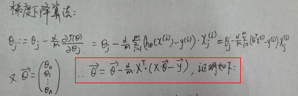
故
3.推导过程


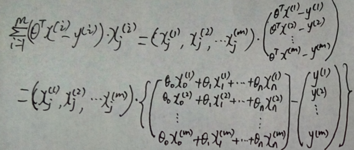
4. theta = theta - (alpha * T) / m;
实际上就是
.实际上T=
经过向量推导后（推导过程见3）第i行，第j列，T=
5. J_history(iter) = computeCost(X, y, theta);

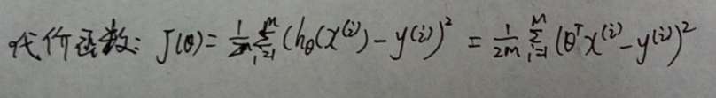
j= sum((X*theta - y).^2) / (2 * m);
6.具体细节先理解到这，慢慢理解不着急，慢慢向前走，一定可以成功！