A wizard’s guide to Adversarial Autoencoders: Part 1, Autoencoder?

“If you know how to write a code to classify MNIST digits using Tensorflow, then you are all set to read the rest of this post or else I’d highly suggest you go through this article on Tensorflow’s website.”

“We know now that we don’t need any big new breakthroughs to get to true AI.

That is completely, utterly, ridiculously wrong. As I’ve said in previous statements: most of human and animal learning is unsupervised learning. If intelligence was a cake, unsupervised learning would be the cake, supervised learning would be the icing on the cake, and reinforcement learning would be the cherry on the cake.

We know how to make the icing and the cherry, but we don’t know how to make the cake. We need to solve the unsupervised learning problem before we can even think of getting to true AI. And that’s just an obstacle we know about. What about all the ones we don’t know about?”

This is a quote from Yan Lecun (I know, another one from Yan Lecun), the director of AI research at Facebook after AlphaGo’s victory.

We know that a Convolutional Neural Networks (CNNs) or in some cases Dense fully connected layers (MLP — Multi layer perceptron as some would like to call it) can be used to perform image recognition. But, a CNN (or MLP) alone cannot be used to perform tasks like content and style separation from an image, generate real looking images (a generative model), classify images using a very small set of labeled or perform data compression (like zipping a file).

Each of these tasks might require its own architecture and training algorithm. But, wouldn’t it be cool if we were able to implement all the above mentioned tasks using just one architecture. An Adversarial Autoencoder (one that trained in a semi-supervised manner) can perform all of them and more using just one architecture.

We’ll build an Adversarial Autoencoder that can compress data (MNIST digits in a lossy way), separate style and content of the digits (generate numbers with different styles), classify them using a small subset of labeled data to get high classification accuracy (about 95% using just 1000 labeled digits!) and finally also act as a generative model (to generate real looking fake digits).

Before we go into the theoretical and the implementation parts of an Adversarial Autoencoder, let’s take a step back and discuss about Autoencoders and have a look at a simple tensorflow implementation.

---

Autoencoder Architecture

An Autoencoder is a neural network that is trained to produce an output which is very similar to its input (so it basically attempts to copy its input to its output) and since it doesn’t need any targets (labels), it can be trained in an unsupervised manner.

It has two parts:

1. Encoder: It takes in an input x (this can be an image, word embeddings, video or audio data) and produces an output h (where h usually has a lower dimensionality than x). For example, the encoder can take in an image x of size 100 x 100 and produce an output h (also known as the latent code) of size 100 x 1 (this can be any size). The encoder in this case just compresses the image such that it’ll occupy a lower dimensional space, on doing so we can now see that h (100 x 1 in size) could be stored using 100 times less memory than directly storing the image x (this will result in some loss of data though).

Let’s think of a compression software like WinRAR (still on a free trial?) which can be used to compress a file to get a zip (or rar,…) file that occupies lower amounts of space. A similar operation is performed by the encoder in an autoencoder architecture.

If the encoder is represented by the function q, then

Encoder

2. Decoder: It takes in the output of an encoder h and tries to reconstruct the input at its output. Continuing from the encoder example, h is now of size 100 x 1, the decoder tries to get back the original 100 x 100 image using h. We’ll train the decoder to get back as much information as possible from h to reconstruct x.

So, the decoder’s operation is similar to performing an unzipping on WinRAR.

If the function p represents our decoder then the reconstructed image x_ is:

Decoder

Dimensionality reduction works only if the inputs are correlated (like images from the same domain). It fails if we pass in completely random inputs each time we train an autoencoder. So in the end, an autoencoder can produce lower dimensional output (at the encoder) given an input much like Principal Component Analysis (PCA). And since we don’t have to use any labels during training, it’s an unsupervised model as well.

---

But, What can Autoencoders be used for other than dimensionality reduction?

• Image denoising wherein a clear noise free image could be generated using a noisy one.

Denoising autoencoder example on handwritten digits. Source: https://www.doc.ic.ac.uk/~js4416/163/website/autoencoders/denoising.html

• Semantic Hashing where dimensionality reduction could be used to make information retrieval faster (I found this very interesting!).
• And recently where Autoencoders trained in an adversarial manner could be used as generative models (We’ll go deeper into this later).

I’ve divided this post into four parts:

• Part 1: Autoencoders?

We’ll start with an implementation of a simple Autoencoder using Tensorflow and reduce the dimensionality of MNIST (You’ll definitely know what this dataset is about) dataset images.

• Part 2: Exploring the latent space with Adversarial Autoencoders.

We’ll introduce constraints on the latent code (output of the encoder) using adversarial learning.

• Part 3: Disentanglement of style and content.

Here we’ll generate different images with the same style of writing.

• Part 4: Classify MNIST with 1000 labels.

We’ll train an AAE to classify MNIST digits to get an accuracy of about 95% using only 1000 labeled inputs (Impressive ah?).

---

Let’s begin Part 1 by having a look at the network architecture we”ll need to implement.

As stated earlier an autoencoder (AE) as two parts an encoder and a decoder, let’s begin with a simple dense fully connected encoder architecture:

Encoder Architecture

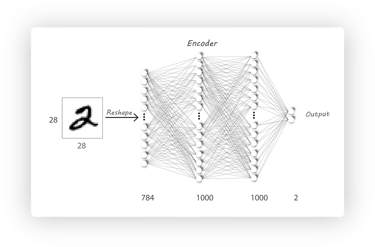
It consists of an input layer with 784 neurons (cause we have flattened the image to have a single dimension), two sets of 1000 ReLU activated neurons form the hidden layers and an output layer consisting of 2 neurons without any activation provides the latent code.

If you just want to get your hands on the code check out this link:

Naresh1318/Adversarial_Autoencoder
Contribute to Adversarial_Autoencoder development by creating an account on GitHub.github.com

To implement the above architecture in Tensorflow we’ll start off with a dense() function which’ll help us build a dense fully connected layer given input x, number of neurons at the input n1 and number of neurons at output n2. The name parameter is used to set a name for variable_scope. More on shared variables and using variable scope can be found here (I’d highly recommend having a look at it).

I’ve used tf.get_variable()instead of tf.Variable()to create the weight and bias variables so that we can later reuse the trained model (either the encoder or decoder alone) to pass in any desired value and have a look at their output.

Next, we’ll use this dense() function to implement the encoder architecture. The code is straight forward, but note that we haven’t used any activation at the output.

• reuse flag is used to reuse the trained encoder architecture.
• here input_dim = 784, n_l1 = 1000, n_l2 = 1000, z_dim = 2 .

The decoder is implemented in a similar manner, the architecture we’ll need is:

Decoder Architecture

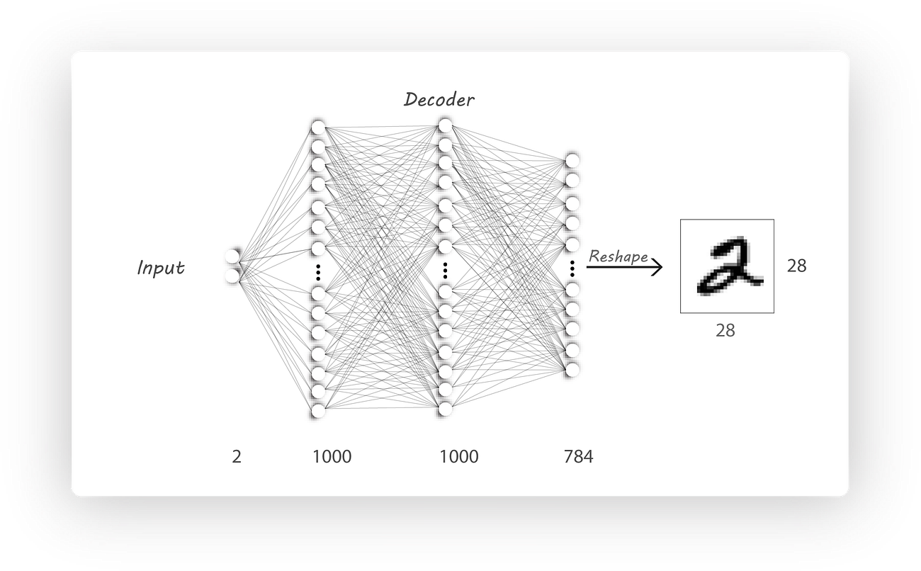
Again we’ll just use the dense() function to build our decoder. However, I’ve used sigmoid activation for the output layer to ensure that the output values range between 0 and 1 (the same range as our input).

• z_dim = 2, n_l2 = 1000, n_l1 = 1000, input_dim = 784 same as the encoder.

The encoder output can be connected to the decoder just like this:

This now forms the exact same autoencoder architecture as shown in the architecture diagram. We’ll pass in the inputs through the placeholder x_input (size: batch_size, 784), set target to be same as x_input and compare the decoder_output to x_input.

The loss function used is the Mean Squared Error (MSE) which finds the distance between the pixels in the input (x_input) and the output image (decoder_output). We call this the reconstruction loss as our main aim is to reconstruct the input at the output.

Mean Squared Error

This is nothing but the mean of the squared difference between the input and the output. which can easily be implemented in Tensorflow as follows:

The optimizer I’ve used is the AdamOptimizer (Feel free to try out new ones, I’ve haven’t experimented on others) with a learning rate of 0.01 and beta1 as 0.9. It’s directly available on Tensorflow and can be used as follows:

Notice that we are backpropagating through both the encoder and the decoder using the same loss function. (I could have changed only the encoder or the decoder weights using the var_list parameter under the minimize()method. Since I haven’t mentioned any, it defaults to all the trainable variables.)

Lastly, we train our model by passing in our MNIST images using a batch size of 100 and using the same 100 images as the target.

The entire code is available on github:

Naresh1318/Adversarial_Autoencoder
Contribute to Adversarial_Autoencoder development by creating an account on GitHub.github.com

Things to note:

• The generate_image_grid() function generates a grid of images by passing a set of numbers to the trained decoder (this is where get_variable comes in handy).
• Each run generates the required tensorboard files under:

./Results/<model>/<time_stamp_and_parameters>/Tensorboard

• The trainig logs are stored in:

./Results/<model>/<time_stamp_and_parameters>/log/log.txt file.

• Set the train flag to True to train the model or set it to False to show the decoder output for some random input.

I’ve trained the model for 200 epochs and shown the variation of loss and the generated images below:

Variation of reconstruction loss

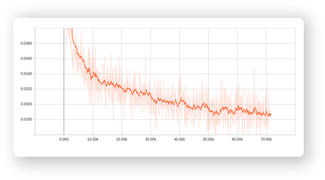
The reconstruction loss is reducing, which just what we want.

Generated Images

Notice how the decoder generalised the output 3 by removing small irregularities like the line on top of the input 3.

Now, what if only consider the trained decoder and pass in some random numbers (I’ve passed 0, 0 as we only have a 2-D latent code) as it’s inputs, we should get some digits right?

Decoder Output at (0, 0)

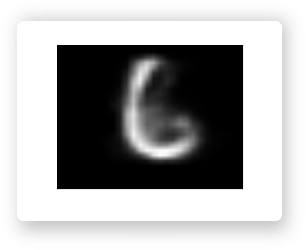
But this doesn’t represent a clear digit at all (well, at least for me).

The reason for this is because the encoder output does not cover the entire 2-D latent space (it has a lot of gaps in its output distribution). So if we feed in values that the encoder hasn’t fed to the decoder during the training phase, we’ll get weird looking output images. This can be overcome by constraining the encoder output to have a random distribution (say normal with 0.0 mean and a standard deviation of 2.0) when producing the latent code. This is exactly what an Adversarial Autoencoder is capable of and we’ll look into its implementation in Part 2.

Have a look at the cover image again!!

Got it?

---

Hope you liked this short article on autoencoders. I would openly encourage any criticism or suggestions to improve my work.

If you think this content is worth sharing hit the ❤️, I like the notifications it sends me!!

原文地址： https://medium.com/towards-data-science/a-wizards-guide-to-adversarial-autoencoders-part-1-autoencoder-d9a5f8795af4