tensorflow 批标准化Batch_normalization

参考链接：https://morvanzhou.github.io/tutorials/machine-learning/tensorflow/5-13-A-batch-normalization/  

首先介绍标准化操作：

平均值为

标准差为 

一般在数据处理之前，对数据做标准化操作。在神经网络中，也可以对隐藏层中的数据进行标准化

举一个比较简单的实例：
在一批数据中，x1=1,x2=20,经过全连接层，Wx1=0.1*1=0.1  Wx2=0.1*20=2,再经过tanh激励函数，tanh(0.1)≈0.1，tanh(20)≈0.96,

近于 1 的部已经处在了 激励函数的饱和阶段, 也就是如果 x 无论再怎么扩大, tanh 激励函数输出值也还是 接近1. 换句话说, 神经网络在初始阶段已经不对那些比较大的 x 特征范围 敏感了. 

BN（batch_normalization）算法

可以使用batch_normalization对隐藏层的数据进行标准化，BN算法下图所示： normalize 后的数据再进行扩展和平移，对γ和 β参数进行反向传播学习，使得处理后的数据达到最佳的使用效果

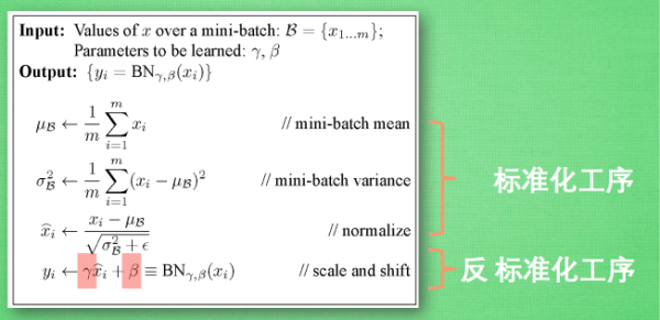
ε是为了防止参数为0

参数反向传播证明：http://blog.csdn.net/UESTC_C2_403/article/details/77365813

实践BN算法：

（1）tf.train.ExponentialMovingAverage(decay, steps)   参考链接：http://blog.csdn.net/uestc_c2_403/article/details/72235334    
tf.train.ExponentialMovingAverage这个函数用于更新参数，就是采用滑动平均move average的方法更新参数。这个函数初始化需要提供一个衰减速率（decay），用于控制模型的更新速度。这个函数还会维护一个影子变量（也就是更新参数后的参数值），这个影子变量的初始值就是这个变量的初始值，影子变量值的更新方式如下：
shadow_variable = decay * shadow_variable + (1-decay) * variable
shadow_variable是影子变量，variable表示待更新的变量，也就是变量被赋予的值，decay为衰减速率。decay一般设为接近于1的数（0.99,0.999）。decay越大模型越稳定，因为decay越大，参数更新的速度就越慢，趋于稳定。
tf.train.ExponentialMovingAverage这个函数还提供了自己动更新decay的计算方式：
decay= min（decay，（1+steps）/（10+steps））
steps是迭代的次数，可以自己设定。

（2）control_dependencies(self, control_inputs)   和 tf.identity(input, name=None) 参考链接：http://blog.csdn.net/winycg/article/details/78820032     

（3）实现BN算法的代码 方法如下：一种使用tf.nn,一种使用tf.layers

① 每批batch的mean和var 都会不同, 所以我们可以使用 moving average 的方法记录并慢慢改进 mean和var 的值. 然后将修改提升后的 mean和var 放入 tf.nn.batch_normalization().

y_mean, y_var = tf.nn.moments(y, axes=[0])update_op = tf.train.ExponentialMovingAverage(decay=0.5).apply([y_mean, y_var])with tf.control_dependencies([update_op]):y_mean2, y_var2 = tf.identity(y_mean), tf.identity(y_var)scale = tf.Variable(tf.ones([out_size]))shift = tf.Variable(tf.zeros([out_size]))eposilon = 0.001y = tf.nn.batch_normalization(y, y_mean2, y_var2, shift, scale, eposilon)# 此函数封装如下操作# y = (y - y_mean) / tf.sqrt(y_var + 0.001)# y = y * scale + shift

②高度集成，参考链接：https://tensorflow.google.cn/api_docs/python/tf/layers/batch_normalization

# 其他参数为默认值，momentum是滑动平均参数tf.layers.batch_normalization(x, momentum=0.4, training=True)

线性回归预测 

为了测试在BN前后的差距，采用tanh作为激励函数

import tensorflow as tfimport numpy as npimport matplotlib.pyplot as pltfrom PIL import Imagen_train_samples = 2000n_test_samples = 200batch_size = 128epoch = 250lr = 0.03n_input = 1n_hidden = 8hidden_size = 10n_output = 1# pre_activation[]记录每层还没有进行标准化和激励函数的值# layer_input[]记录每层激励函数之后的结果class NN(object):    def __init__(self, is_bn=False):        # 在类内创建属于自己的计算图        self.gra = tf.Graph()        with self.gra.as_default():            self.n_input = n_input            self.n_hidden = n_hidden            self.n_output = n_output            self.hidden_size = hidden_size            self.is_bn = is_bn            self.x_data = tf.placeholder(tf.float32, [None, self.n_input])            self.y_data = tf.placeholder(tf.float32, [None, self.n_output])            self.is_training = tf.placeholder(tf.bool)            self.pre_activation = []            self.w_init = tf.random_normal_initializer(0, 0.1)            self.b_init = tf.zeros_initializer()            self.layer_input = []            self.pre_activation.append(self.x_data)            if self.is_bn:                self.layer_input.append(                    tf.layers.batch_normalization(self.x_data, training=self.is_training))            else:                self.layer_input.append(self.x_data)            for i in range(self.n_hidden):                self.layer_input.append(self.add_layer(self.layer_input[-1],                                                       out_size=self.hidden_size,                                                        activation_function=tf.nn.tanh))            self.y = tf.layers.dense(self.layer_input[-1],                                      self.n_output,                                     kernel_initializer=self.w_init,                                      bias_initializer=self.b_init)            self.loss = tf.losses.mean_squared_error(self.y_data, self.y)            # 若操作中存在batch_normalization，滑动平均和滑动方差更新操作存在于GraphKeys.UPDATE_OPS            # 训练之前需要先执行更新操作            update_ops = tf.get_collection(tf.GraphKeys.UPDATE_OPS)            with tf.control_dependencies(update_ops):                self.train_step = tf.train.AdamOptimizer(lr).minimize(self.loss)            init = tf.global_variables_initializer()        self.sess = tf.Session(graph=self.gra)        self.sess.run(init)    def add_layer(self, x, out_size, activation_function=None):        x = tf.layers.dense(x, out_size, kernel_initializer=self.w_init, bias_initializer=self.b_init)        self.pre_activation.append(x)        if self.is_bn:            x = tf.layers.batch_normalization(x, momentum=0.4, training=self.is_training)        if activation_function is None:            output = x        else:            output = activation_function(x)        return output    def run_train_step(self, tf_x, tf_y, is_train):        self.sess.run(self.train_step,                      feed_dict={self.x_data: tf_x, self.y_data: tf_y, self.is_training: is_train})    def run_out(self, tf_x, is_train):        return self.sess.run(self.y,                             feed_dict={self.x_data: tf_x, self.is_training: is_train})    def run_loss_input(self, tf_x, tf_y, is_train):        return self.sess.run([self.loss, self.layer_input, self.pre_activation],                             feed_dict={self.x_data: tf_x, self.y_data: tf_y, self.is_training: is_train})# 产生train数据train_x = np.linspace(-7, 10, n_train_samples)[:, np.newaxis]# 产生数据之后要打乱一下，否则神经网络每次学习的是一段局部曲线，# 而每段曲线之间可能是差异很大的，就会影响神经网络的判断np.random.shuffle(train_x)noise = np.random.normal(0, 0.2, train_x.shape)train_y = np.square(train_x) + noise# 产生test数据test_x = np.linspace(-7, 10, n_test_samples)[:, np.newaxis]noise = np.random.normal(0, 0.2, test_x.shape)test_y = np.square(test_x) + noise# 随机获取数据def get_random_data_block(data_x, data_y, data_batch_size):    index = np.random.randint(0, len(data_x) - data_batch_size)    return data_x[index: index + data_batch_size], data_y[index: index + data_batch_size]# 建立用于对比的神经网络nn_bn = NN(is_bn=True)nn = NN(is_bn=False)fig, axes = plt.subplots(4, n_hidden + 1, figsize=(10, 7), dpi=60)def plot_histogram(l_in, l_in_bn, pre_ac, pre_ac_bn):    for i in range(n_hidden + 1):        # 清空        for j in range(4):            axes[j][i].clear()        #        if i == 0:            p_range = (-7, 10)            the_range = (-7, 10)        else:            p_range = (-4, 4)            the_range = (-1, 1)        axes[0, i].set_title('L' + str(i))        axes[0, i].hist(pre_ac[i].ravel(), bins=10, range=p_range, alpha=0.75)        axes[1, i].hist(pre_ac_bn[i].ravel(), bins=10, range=p_range, alpha=0.75)        axes[2, i].hist(l_in[i].ravel(), bins=10, range=the_range, alpha=0.75)        axes[3, i].hist(l_in_bn[i].ravel(), bins=10, range=the_range, alpha=0.75)        # 将坐标轴的标识清空        for j in range(4):            axes[j, i].set_yticks(())            axes[j, i].set_xticks(())        axes[1, i].set_xticks(p_range)        axes[3, i].set_xticks(the_range)        axes[2, 0].set_ylabel('ACT')        axes[3, 0].set_ylabel('ACT_BN')    plt.pause(0.01)    # 保存每次出现的图像，以便生成gif    global gif_image_num    gif_image_num += 1    plt.savefig(str(gif_image_num) + '.jpg')losses = []losses_bn = []gif_image_num = 0for k in range(epoch):    print(k)    batch_x, batch_y = get_random_data_block(train_x, train_y, batch_size)    nn.run_train_step(batch_x, batch_y, True)    nn_bn.run_train_step(batch_x, batch_y, True)    if k % 10 == 0:        loss, layer_in, pre_activation = nn.run_loss_input(test_x, test_y, False)        loss_bn, layer_in_bn, pre_activation_bn = nn_bn.run_loss_input(test_x, test_y, False)        losses.append(loss)        losses_bn.append(loss_bn)        plot_histogram(layer_in, layer_in_bn, pre_activation, pre_activation_bn)plt.tight_layout()# 利用PIL库生成gif# http://pillow.readthedocs.io/en/latest/handbook/image-file-formats.html#savingbegin_image = Image.open('1.jpg')images = []for num in range(gif_image_num):    if num == 0:        continue    images.append(Image.open(str(num) + '.jpg'))begin_image.save('BN.gif', save_all=True, append_images=images, duration=100)# 绘制loss曲线plt.figure(2)plt.plot(losses, label='NN')plt.plot(losses_bn, label='NN_BN')plt.ylabel('loss')plt.legend()# 绘制预测曲线pred = nn.run_out(test_x, False)pred_bn = nn_bn.run_out(test_x, False)plt.figure(3)plt.plot(test_x, pred, lw=3, label='NN')plt.plot(test_x, pred_bn, lw=3, label='NN_BN')plt.scatter(test_x, test_y, s=10, color='red', alpha=0.3)plt.legend()plt.show()

查看输出值的分布：

误差曲线：

测试数据：