Pandas 数据处理（下）

来源：互联网发布：用手机怎么改淘宝好编辑：程序博客网时间：2024/05/21 10:59

Pandas 数据处理（下）

数值运算

统计

运算通常会排除缺省项

求平均值：

df.mean()

输出：

A   -0.004474B   -0.383981C   -0.687758D    5.000000F    3.000000dtype: float64

求指定轴上的平均值

df.mean(1)

输出：

2013-01-01    0.8727352013-01-02    1.4316212013-01-03    0.7077312013-01-04    1.3950422013-01-05    1.8836562013-01-06    1.592306Freq: D, dtype: float64

不同维度的 pandas 对象也可以做运算，它会自动进行对应，shift 用来做对齐操作。

s = pd.Series([1,3,5,np.nan,6,8], index=dates).shift(2)s

输出：

2013-01-01   NaN2013-01-02   NaN2013-01-03     12013-01-04     32013-01-05     52013-01-06   NaNFreq: D, dtype: float64

对不同维度的 pandas 对象进行减法操作：

df.sub(s, axis='index')

输出：

                   A         B         C   D   F2013-01-01       NaN       NaN       NaN NaN NaN2013-01-02       NaN       NaN       NaN NaN NaN2013-01-03 -1.861849 -3.104569 -1.494929   4   12013-01-04 -2.278445 -3.706771 -4.039575   2   02013-01-05 -5.424972 -4.432980 -4.723768   0  -12013-01-06       NaN       NaN       NaN NaN NaN

函数应用

对数据应用 numpy 函数：

df.apply(np.cumsum) #累加

输出：

                   A         B         C   D   F2013-01-01  0.000000  0.000000 -1.509059   5 NaN2013-01-02  1.212112 -0.173215 -1.389850  10   12013-01-03  0.350263 -2.277784 -1.884779  15   32013-01-04  1.071818 -2.984555 -2.924354  20   62013-01-05  0.646846 -2.417535 -2.648122  25  102013-01-06 -0.026844 -2.303886 -4.126549  30  15

应用自定义函数：

df.apply(lambda x: x.max() - x.min())

输出：

A    2.073961B    2.671590C    1.785291D    0.000000F    4.000000dtype: float64

直方图

对不同值的数量进行统计

s = pd.Series(np.random.randint(0, 7, size=10))s

输出：

0    41    22    13    24    65    46    47    68    49    4dtype: int32

输入：

s.value_counts()

输出：

4    56    22    21    1dtype: int64String Methods

字符处理

s = pd.Series(['A', 'B', 'C', 'Aaba', 'Baca', np.nan, 'CABA', 'dog', 'cat'])s.str.lower()

输出：

0       a1       b2       c3    aaba4    baca5     NaN6    caba7     dog8     catdtype: object

合并

Concat

使用 concat() 连接 pandas 对象:

df = pd.DataFrame(np.random.randn(10, 4))df

输出：

          0         1         2         30 -0.548702  1.467327 -1.015962 -0.4830751  1.637550 -1.217659 -0.291519 -1.7455052 -0.263952  0.991460 -0.919069  0.2660463 -0.709661  1.669052  1.037882 -1.7057754 -0.919854 -0.042379  1.247642 -0.0099205  0.290213  0.495767  0.362949  1.5481066 -1.131345 -0.089329  0.337863 -0.9458677 -0.932132  1.956030  0.017587 -0.0166928 -0.575247  0.254161 -1.143704  0.2158979  1.193555 -0.077118 -0.408530 -0.862495

切片

pieces = [df[:3], df[3:7], df[7:]]pd.concat(pieces)

输出：

          0         1         2         30 -0.548702  1.467327 -1.015962 -0.4830751  1.637550 -1.217659 -0.291519 -1.7455052 -0.263952  0.991460 -0.919069  0.2660463 -0.709661  1.669052  1.037882 -1.7057754 -0.919854 -0.042379  1.247642 -0.0099205  0.290213  0.495767  0.362949  1.5481066 -1.131345 -0.089329  0.337863 -0.9458677 -0.932132  1.956030  0.017587 -0.0166928 -0.575247  0.254161 -1.143704  0.2158979  1.193555 -0.077118 -0.408530 -0.862495

Join

SQL 风格的合并

left = pd.DataFrame({'key': ['foo', 'foo'], 'lval': [1, 2]})right = pd.DataFrame({'key': ['foo', 'foo'], 'rval': [4, 5]})

输入：

left

输出：

   key  lval0  foo     11  foo     2

输入：

right

输出：

   key  rval0  foo     41  foo     5

输入：

pd.merge(left, right, on=’key’)

输出：

   key  lval  rval0  foo     1     41  foo     1     52  foo     2     43  foo     2     5

追加

在 dataframe 数据后追加行

df = pd.DataFrame(np.random.randn(8, 4), columns=['A','B','C','D'])df

输出：

          A         B         C         D0  1.346061  1.511763  1.627081 -0.9905821 -0.441652  1.211526  0.268520  0.0245802 -1.577585  0.396823 -0.105381 -0.5325323  1.453749  1.208843 -0.080952 -0.2646104 -0.727965 -0.589346  0.339969 -0.6932055 -0.339355  0.593616  0.884345  1.5914316  0.141809  0.220390  0.435589  0.1924517 -0.096701  0.803351  1.715071 -0.708758

输入：

s = df.iloc[3]df.append(s, ignore_index=True)

输出：

          A         B         C         D0  1.346061  1.511763  1.627081 -0.9905821 -0.441652  1.211526  0.268520  0.0245802 -1.577585  0.396823 -0.105381 -0.5325323  1.453749  1.208843 -0.080952 -0.2646104 -0.727965 -0.589346  0.339969 -0.6932055 -0.339355  0.593616  0.884345  1.5914316  0.141809  0.220390  0.435589  0.1924517 -0.096701  0.803351  1.715071 -0.7087588  1.453749  1.208843 -0.080952 -0.264610

分组

分组常常意味着可能包含以下的几种的操作中一个或多个

依据一些标准分离数据
对组单独地应用函数
将结果合并到一个数据结构中

输入：

df = pd.DataFrame({'A' : ['foo', 'bar', 'foo', 'bar',                          'foo', 'bar', 'foo', 'foo'],                   'B' : ['one', 'one', 'two', 'three',                          'two', 'two', 'one', 'three'],                   'C' : np.random.randn(8),                   'D' : np.random.randn(8)})df

输出：

     A      B         C         D0  foo    one -1.202872 -0.0552241  bar    one -1.814470  2.3959852  foo    two  1.018601  1.5528253  bar  three -0.595447  0.1665994  foo    two  1.395433  0.0476095  bar    two -0.392670 -0.1364736  foo    one  0.007207 -0.5617577  foo  three  1.928123 -1.623033

对单个分组应用函数，数据被分成了 bar 组与 foo 组，分别计算总和。

df.groupby('A').sum()

输出：

            C        DA                     bar -2.802588  2.42611foo  3.146492 -0.63958

依据多个列分组会构成一个分级索引：

df.groupby(['A','B']).sum()

输出：

                  C         DA   B                        bar one   -1.814470  2.395985    three -0.595447  0.166599    two   -0.392670 -0.136473foo one   -1.195665 -0.616981    three  1.928123 -1.623033    two    2.414034  1.600434

数据透视表

df = pd.DataFrame({'A' : ['one', 'one', 'two', 'three'] * 3,                   'B' : ['A', 'B', 'C'] * 4,                   'C' : ['foo', 'foo', 'foo', 'bar', 'bar', 'bar'] * 2,                   'D' : np.random.randn(12),                   'E' : np.random.randn(12)})df

输出：

        A  B    C         D         E0     one  A  foo  1.418757 -0.1796661     one  B  foo -1.879024  1.2918362     two  C  foo  0.536826 -0.0096143   three  A  bar  1.006160  0.3921494     one  B  bar -0.029716  0.2645995     one  C  bar -1.146178 -0.0574096     two  A  foo  0.100900 -1.4256387   three  B  foo -1.035018  1.0240988     one  C  foo  0.314665 -0.1060629     one  A  bar -0.773723  1.82437510    two  B  bar -1.170653  0.59597411  three  C  bar  0.648740  1.167115

生成数据透视表：

pd.pivot_table(df, values='D', index=['A', 'B'], columns=['C'])

输出：

C             bar       fooA     B                    one   A -0.773723  1.418757      B -0.029716 -1.879024      C -1.146178  0.314665three A  1.006160       NaN      B       NaN -1.035018      C  0.648740       NaNtwo   A       NaN  0.100900      B -1.170653       NaN      C       NaN  0.536826

时间序列

pandas 拥有既简单又强大的频率变换重新采样功能，下面的例子从 1次/秒转换到了 1次/5分钟：

rng = pd.date_range('1/1/2012', periods=100, freq='S')ts = pd.Series(np.random.randint(0, 500, len(rng)), index=rng)ts.resample('5Min', how='sum')

输出：

2012-01-01    25083Freq: 5T, dtype: int32

本地化时区表示

rng = pd.date_range('3/6/2012 00:00', periods=5, freq='D')ts = pd.Series(np.random.randn(len(rng)), rng)ts

输出：

2012-03-06    0.4640002012-03-07    0.2273712012-03-08   -0.4969222012-03-09    0.3063892012-03-10   -2.290613Freq: D, dtype: float64

输入：

ts_utc = ts.tz_localize('UTC')ts_utc

输出：

2012-03-06 00:00:00+00:00    0.4640002012-03-07 00:00:00+00:00    0.2273712012-03-08 00:00:00+00:00   -0.4969222012-03-09 00:00:00+00:00    0.3063892012-03-10 00:00:00+00:00   -2.290613Freq: D, dtype: float64

转化成其他时区

ts_utc.tz_convert('US/Eastern')

输出：

2012-03-05 19:00:00-05:00    0.4640002012-03-06 19:00:00-05:00    0.2273712012-03-07 19:00:00-05:00   -0.4969222012-03-08 19:00:00-05:00    0.3063892012-03-09 19:00:00-05:00   -2.290613Freq: D, dtype: float64

时间跨度的转换

rng = pd.date_range('1/1/2012', periods=5, freq='M')ts = pd.Series(np.random.randn(len(rng)), index=rng)ts

输出：

2012-01-31   -1.1346232012-02-29   -1.5618192012-03-31   -0.2608382012-04-30    0.2819572012-05-31    1.523962Freq: M, dtype: float64

转换为周期

ps = ts.to_period()ps

输出：

2012-01   -1.1346232012-02   -1.5618192012-03   -0.2608382012-04    0.2819572012-05    1.523962Freq: M, dtype: float64

转换为时间戳

ps.to_timestamp()

输出：

2012-01-01   -1.1346232012-02-01   -1.5618192012-03-01   -0.2608382012-04-01    0.2819572012-05-01    1.523962Freq: MS, dtype: float64

在周期与时间戳之间进行转换这一功能对一些算术函数很有用，在下面的例子中我们改变时间序列的相位。

prng = pd.period_range('1990Q1', '2000Q4', freq='Q-NOV')ts = pd.Series(np.random.randn(len(prng)), prng)ts.index = (prng.asfreq('M', 'e') + 1).asfreq('H', 's') + 9ts.head()

输出：

1990-03-01 09:00   -0.9029371990-06-01 09:00    0.0681591990-09-01 09:00   -0.0578731990-12-01 09:00   -0.3682041991-03-01 09:00   -1.144073Freq: H, dtype: float64

分类

df = pd.DataFrame({"id":[1,2,3,4,5,6], "raw_grade":['a', 'b', 'b', 'a', 'a', 'e']})

将 raw_grades 转换成 Categoricals 类型。

df["grade"] = df["raw_grade"].astype("category")df["grade"]

输出：

0    a1    b2    b3    a4    a5    eName: grade, dtype: categoryCategories (3, object): [a, b, e]

重命名分类

df["grade"].cat.categories = ["very good", "good", "very bad"]

对分类进行重排序，同时加入新的分类。

df["grade"] = df["grade"].cat.set_categories(["very bad", "bad", "medium", "good", "very good"])df["grade"]

输出：

0    very good1         good2         good3    very good4    very good5     very badName: grade, dtype: categoryCategories (5, object): [very bad, bad, medium, good, very good]

根据分类的顺序对数据进行排序

df.sort("grade")

输出：

   id raw_grade      grade5   6         e   very bad1   2         b       good2   3         b       good0   1         a  very good3   4         a  very good4   5         a  very good

按类别分组

df.groupby("grade").size()

输出：

gradevery bad      1bad         NaNmedium      NaNgood          2very good     3dtype: float64

作图

ts = pd.Series(np.random.randn(1000), index=pd.date_range('1/1/2000', periods=1000))ts = ts.cumsum()ts.plot()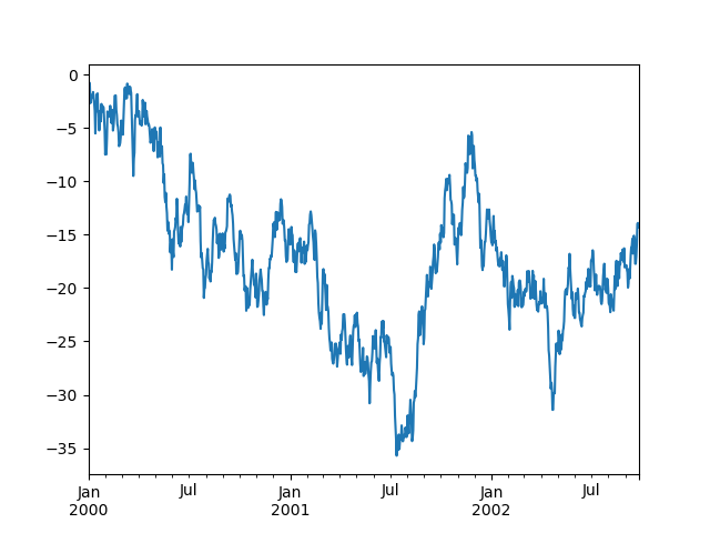

在 DataFrame 中, plot() 可以很方便地为所有列作图:

df = pd.DataFrame(np.random.randn(1000, 4), index=ts.index,                  columns=['A', 'B', 'C', 'D'])df = df.cumsum()plt.figure(); df.plot(); plt.legend(loc='best')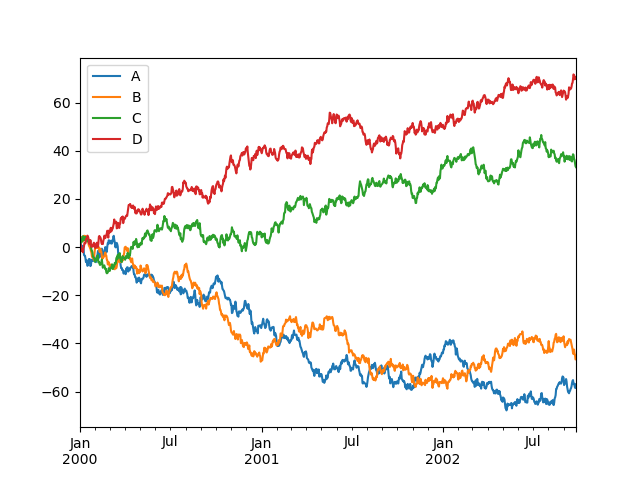

数据 I/O

CSV

保存到 csv 文件

df.to_csv('foo.csv')

从 csv 文件读取数据

pd.read_csv('foo.csv')

输出：

     Unnamed: 0          A          B         C          D0    2000-01-01   0.266457  -0.399641 -0.219582   1.1868601    2000-01-02  -1.170732  -0.345873  1.653061  -0.2829532    2000-01-03  -1.734933   0.530468  2.060811  -0.5155363    2000-01-04  -1.555121   1.452620  0.239859  -1.1568964    2000-01-05   0.578117   0.511371  0.103552  -2.4282025    2000-01-06   0.478344   0.449933 -0.741620  -1.9624096    2000-01-07   1.235339  -0.091757 -1.543861  -1.084753..          ...        ...        ...       ...        ...993  2002-09-20 -10.628548  -9.153563 -7.883146  28.313940994  2002-09-21 -10.390377  -8.727491 -6.399645  30.914107995  2002-09-22  -8.985362  -8.485624 -4.669462  31.367740996  2002-09-23  -9.558560  -8.781216 -4.499815  30.518439997  2002-09-24  -9.902058  -9.340490 -4.386639  30.105593998  2002-09-25 -10.216020  -9.480682 -3.933802  29.758560999  2002-09-26 -11.856774 -10.671012 -3.216025  29.369368[1000 rows x 5 columns]

Excel

保存到 excel 文件

df.to_excel('foo.xlsx', sheet_name='Sheet1')

读取 excel 文件

pd.read_excel('foo.xlsx', 'Sheet1', index_col=None, na_values=['NA'])                    A          B         C          D2000-01-01   0.266457  -0.399641 -0.219582   1.1868602000-01-02  -1.170732  -0.345873  1.653061  -0.2829532000-01-03  -1.734933   0.530468  2.060811  -0.5155362000-01-04  -1.555121   1.452620  0.239859  -1.1568962000-01-05   0.578117   0.511371  0.103552  -2.4282022000-01-06   0.478344   0.449933 -0.741620  -1.9624092000-01-07   1.235339  -0.091757 -1.543861  -1.084753...               ...        ...       ...        ...2002-09-20 -10.628548  -9.153563 -7.883146  28.3139402002-09-21 -10.390377  -8.727491 -6.399645  30.9141072002-09-22  -8.985362  -8.485624 -4.669462  31.3677402002-09-23  -9.558560  -8.781216 -4.499815  30.5184392002-09-24  -9.902058  -9.340490 -4.386639  30.1055932002-09-25 -10.216020  -9.480682 -3.933802  29.7585602002-09-26 -11.856774 -10.671012 -3.216025  29.369368[1000 rows x 4 columns]

License

本作品在知识共享许可协议3.0 下许可授权。

0 0