可视化深度学习和人类感知Visualizing Representations: Deep Learning and Human Beings-2

Example 3: Translation Model

The previous two examples have been, while fun, kind of strange. They were both produced by networks doing simple contrived tasks that we don’t actually care about, with the goal of creating nice representations. The representations they produce are really cool and useful… But they don’t do too much to validate our approach to understanding neural networks.

Let’s look at a cutting edge network doing a real task: translating English to French.

Sutskever et al. (2014) translate English sentences into French sentences using two recurrent neural networks. The first consumes the English sentence, word by word, to produce a representation of it, and the second takes the representation of the English sentence and sequentially outputs translated words. The two are jointly trained, and use a multilayered Long Short Term Memory architecture.3

We can look at the representation right after the English “end of sentence” (EOS) symbol to get a representation of the English sentence. This representation is actually quite a remarkable thing. Somehow, from an English sentence, we’ve formed a vector that encodes the information we need to create a French version of that sentence.

Let’s give this representation a closer look with t-SNE.

Color sentences by first word (eg. The): 

Translation representation of sentences visualized with t-SNE
(Hover over a point to see the sentence.)

This visualization revealed something that was fairly surprising to us: the representation is dominated by the first word.

If you look carefully, there’s a bit more structure than just that. In some places, we can see subclusters corresponding to the second word (for example, in the quotes cluster, we see subclusters for “I” and “We”). In other places we can see sentences with similar first words mix together (eg. “This” and “That”). But by and large, the sentence representation is controlled by the first word.

There are a few reasons this might be the case. The first is that, at the point we grab this representation, the network is giving the first translated word, and so the representation may strongly emphasize the information it needs at that instant. It’s also possible that the first word is much harder than the other words to translate because, for the other words, it is allowed to know what the previous word in the translation was and can kind of Markov chain along.

Still, while there are reasons for this to be the case, it was pretty surprising. I think there must be lots of cases like this, where a quick visualization would reveal surprising insights into the models we work with. But, because visualization is inconvenient, we don’t end up seeing them.

Aside: Patterns for Visualizing High-Dimensional Data

There are a lot of established best practices for visualizing low dimensional data. Many of these are even taught in school. “Label your axes.” “Put units on the axes.” And so on. These are excellent practices for visualizing and communicating low-dimensional data.

Unfortunately, they aren’t as helpful when we visualize high-dimensional data. Label the axes of a t-SNE plot? The axes don’t really have any meaning, nor are the units very meaningful. The only really meaningful thing, in a t-SNE plot, is which points are close together.

There are also some unusual challenges when doing t-SNE plots. Consider the following t-SNE visualization of word embeddings. Look at the cluster of male names on the left hand side…

A Word Embedding Visualized with t-SNE
(This visualization is deliberately terrible.)

… but you can’t look at the cluster of male names on the left hand side. (It’s frustrating not to be able to hover, isn’t it?) While the points are in the exact same positions as in our earlier visualization, without the ability to look at which words correspond to points, this plot is essentially useless. At best, we can look at it and say that the data probably isn’t random.

The problem is that in dimensionality reduced plots of high-dimensional data, position doesn’t explain the data points. This is true even if you understand precisely what the plot you are looking at is.

Well, we can fix that. Let’s add back in the tooltip. Now, by hovering over points you can see what word the correspond to. Why don’t you look at the body part cluster?

A Word Embedding Visualized with t-SNE
(This visualization is deliberately terrible, but less than the previous one.)

You are forgiven if you didn’t have the patience to look at several hundred data points in order to find the body part cluster. And, unless you remembered where it was from before, that’s the effort one would expect it to take you.

The ability to inspect points is not sufficient. When dealing with thousands of points, one needs a way to quickly get a high-level view of the data, and then drill in on the parts that are interesting.

This brings us to my personal theory of visualizing high dimensional data (based on my whole three months of working on visualizing it):

1. There must be a way to interrogate individual data points.
2. There must be a way to get a high-level view of the data.

Interactive visualizations are a really easy way to get both of these properties. But they aren’t the only way. There’s a really beautiful visualization of MNIST in the original t-SNE paper,Maaten & Hinton (2008), on the page labeled 2596:

MNIST Visualized with t-SNE
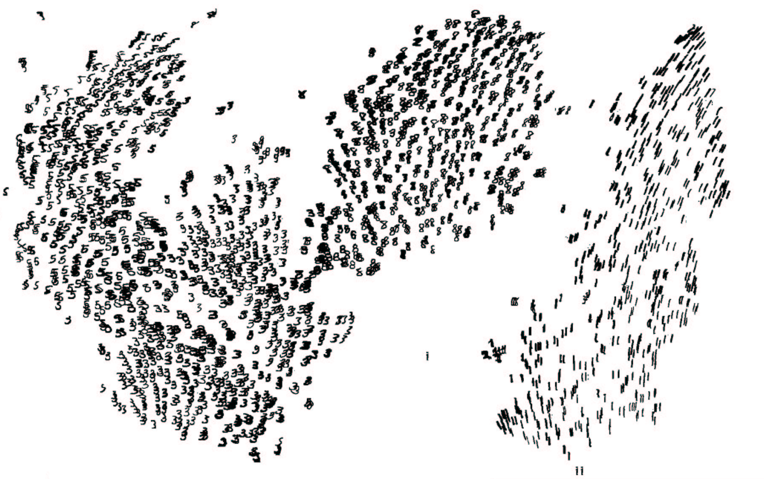
(partial image from Maaten & Hinton (2008))

By directly embedding every MNIST digit’s image in the visualization, Maaten and Hinton made it very easy to inspect individual points. Further, from the ‘texture’ of clusters, one can also quickly recognize their nature.

Unfortunately, that approach only works because MNIST images are small and simple. In their exciting paper on phrase representations, Cho et al. (2014) include some very small subsections of a t-SNE visualization of phrases:

Phrases Visualized with t-SNE
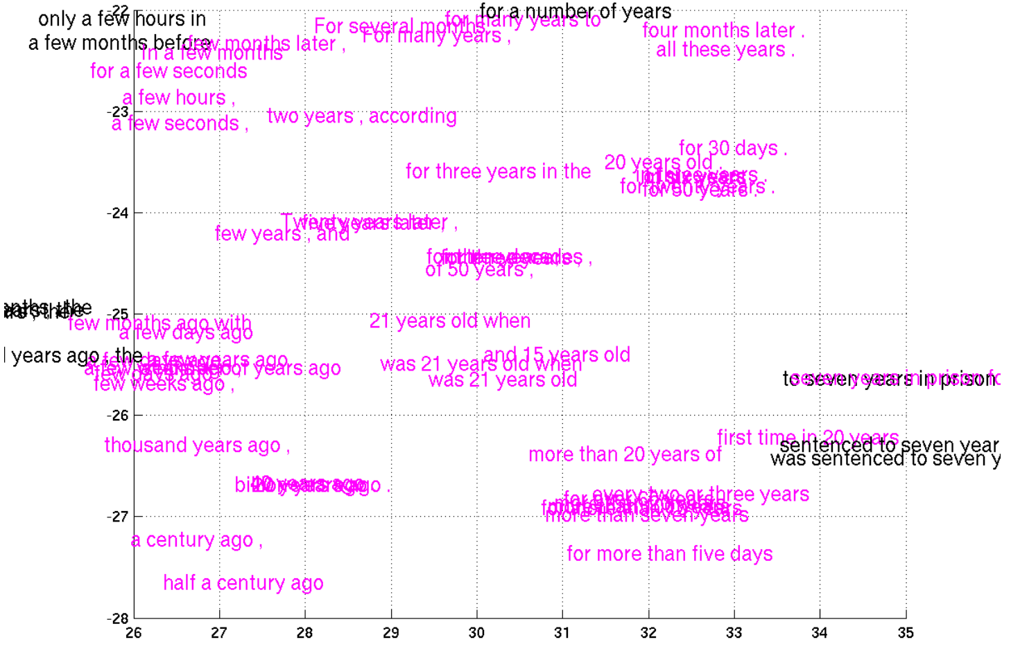
(from Cho et al. (2014))

Unfortunately, embedding the phrases directly in the visualization just doesn’t work. They’re too large and clunky. Actually, I just don’t see any good way to visualize this data without using interactive media.

Geometric Fingerprints

Now that we’ve looked at a bunch of exciting representations, let’s return to our simple MNIST networks and examine the representations they form. We’ll use PCA for dimensionality reduction now, since it will allow us to observe some interesting geometric properties of these representations, and because it is less stochastic than the other dimensionality reduction algorithms we’ve discussed.

The following network has a 5 unit sigmoid layer. Such a network would never be used in practice, but is a bit fun to look at.

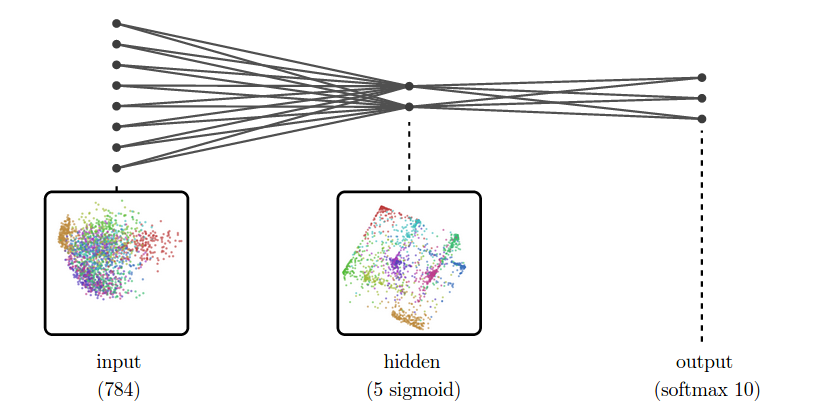
Then network’s hidden representation looks like a projection of a high-dimensional cube. Why? Well, sigmoid units tend to give values close to 0 or 1, and less frequently anything in the middle. If you do that in a bunch of dimensions, you end up with concentration at the corners of a high-dimensional cube and, to a lesser extent, along its edges. PCA then projects this down into two dimensions.

This cube-like structure is a kind of geometric fingerprint of sigmoid layers. Do other activation functions have a similar geometric fingerprint? Let’s look at a ReLU layer.

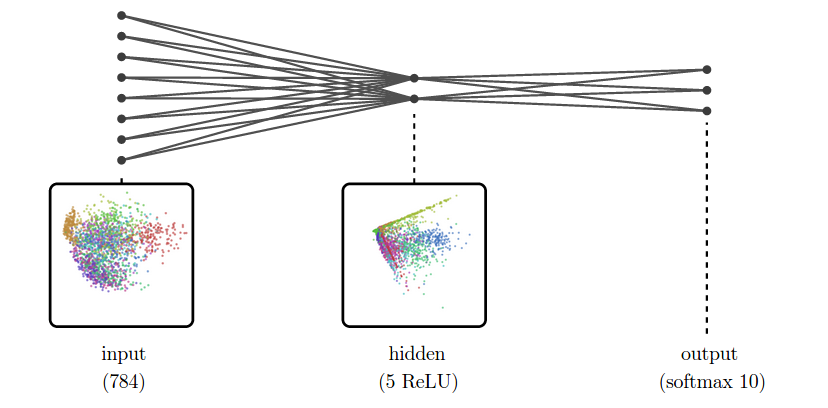
Because ReLU’s have a high probability of being zero, lots of points concentrate on the origin, and along axes. Projected into two dimensions, it looks like a bunch of “spouts” shooting out from the origin.

These geometric properties are much more visible when there are only a few neurons.

from: http://colah.github.io/posts/2015-01-Visualizing-Representations/