caffe2--Toy Regression(五)

Toy Regression

怎么样用caffe2特征实现简单的线性回归：

• 随机生成一些样本数据作为模型的输入
• 用这些数据创建一个网络
• 自动训练模型

• 使用SGD算法优化网络学习的参数

  Browse the Tutorial

  输入两维的X，一维的输出y，权重向量w=[2.0,1.5],偏置b=0.5，方程式：

  y=wx+b
  在本教程中，我们将使用Caffe2运算符生成训练数据。 请注意，您的日常培训工作通常不是这样：在真正场景中的训练数据通常从外部来源加载，例如Caffe DB（即键值存储）或Hive tabel。 我们将在MNIST教程中介绍。

from caffe2.python import core ,cnn, net_drawer, workspace, visualizeimport numpy as npfrom IPython import displayfrom matplotlib import pyplot

---

声明计算图

我们声明有两个图：一个用于初始化我们将在计算中使用的不同参数和常量；另一个是使用随机梯度下降的主图。

第一，初始化网络：注意它的名字不重要，我们基本上想把初始化代码放在一个网中，所以，我们可以调用RunNetOnce()来执行它。分开初始化init_net的原因是，这些operators在训练过程中不需要运行多次。

init_net=core.Net("init")#The ground truth parametersW_gt=init_net.GivenTensorFill(    [],"W_gt",shape=[1,2] ,values=[2.0,1.5])B_gt=init_net.GivenTensorFill([],"B_gt",shape=[1],values=[0.5])#Constant value ONE is used in weighted sum when updating parameters.ONE=init_net.ConstantFill([],"ONE",shape=[1],value=1.)#ITER is the iterator countITER=init_net.ConstantFill([],"ITER",shape=[1],value=0,dtype=core.DataType.INT32)#For the parameters to be learned: we randomly initialize weight#from [-1,1]and init bias with 0.0.W=init_net.UniformFill([], "W", shape=[1,2], min=-1, max=1.)B=init_net.ConstantFill([], "B",  shape=[1],value=0.0)print("Created init net.")

Created init net.

训练网络定义如下：

• 前向传播计算loss
• 通过自动微分计算反向传播
• 使用标准的SGD更新参数

train_net = core.Net("train")# First, we generate random samples of X and create the ground truth.X = train_net.GaussianFill([], "X", shape=[64, 2], mean=0.0, std=1.0, run_once=0)Y_gt = X.FC([W_gt, B_gt], "Y_gt")# We add Gaussian noise to the ground truthnoise = train_net.GaussianFill([], "noise", shape=[64, 1], mean=0.0, std=1.0, run_once=0)Y_noise = Y_gt.Add(noise, "Y_noise")# Note that we do not need to propagate the gradients back through Y_noise,# so we mark StopGradient to notify the auto differentiating algorithm# to ignore this path.Y_noise = Y_noise.StopGradient([], "Y_noise")# Now, for the normal linear regression prediction, this is all we need.Y_pred = X.FC([W, B], "Y_pred")# The loss function is computed by a squared L2 distance, and then averaged# over all items in the minibatch.dist = train_net.SquaredL2Distance([Y_noise, Y_pred], "dist")loss = dist.AveragedLoss([], ["loss"])

看一下整个网络是什么样的。从下图中，你可以发现网络主要是四个部分组成的：

1. 随机生成批次的X（GaussianFill生成X）
2. 使用W_gt,B_gt和FC运算符生成Y_gt
3. 使用目前的参数W和B来预测Y_pred
4. 计算loss

graph=net_drawer.GetPydotGraph(train_net.Proto().op,"train",rankdir="LR")display.Image(graph.create_png(),width=800)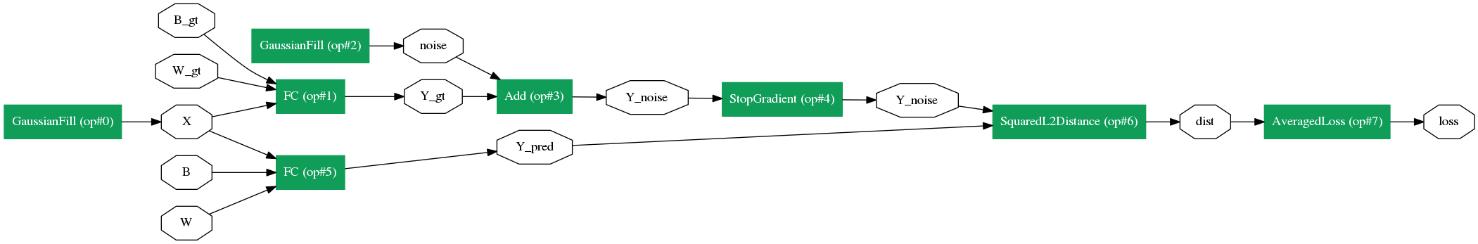

与其它框架相似，caffe2允许我们自动生成梯度运算符，看一下网络模型变成什么样子：

#Get gradients for all the computation abovegradient_map=train_net.AddGradientOperators([loss])graph = net_drawer.GetPydotGraph(train_net.Proto().op, "train", rankdir="LR")display.Image(graph.create_png(),width=800)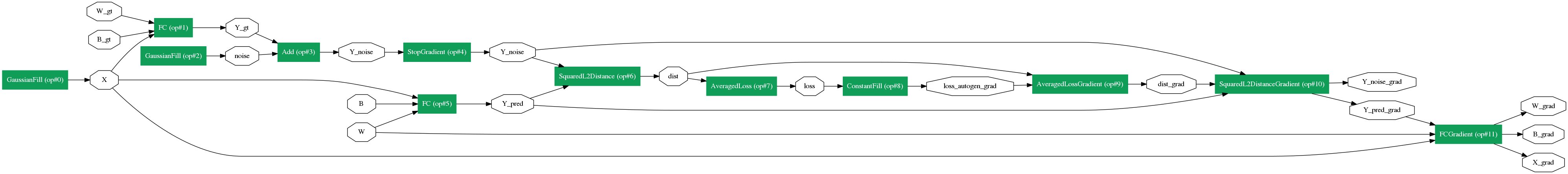

一旦我们得到参数的梯度，我们将添加图的SGD部分：获取当前步骤的学习速率，然后进行参数更新。 在这个例子中，我们并不做任何花哨的东西：只是简单的SGD。

#Increment the iteration by one train_net.Iter(ITER,ITER)#compute the learning rate that corresponds to the iterationLR=train_net.LearningRate(ITER,'LR",base_lr=-0.1,policy="step",stepsize=20,gamma=0.9)# Weighted sumtrain_net.WeightedSum([W, ONE, gradient_map[W], LR], W)train_net.WeightedSum([B, ONE, gradient_map[B], LR], B)# Let's show the graph again.graph = net_drawer.GetPydotGraph(train_net.Proto().op, "train", rankdir="LR")display.Image(graph.create_png(), width=800)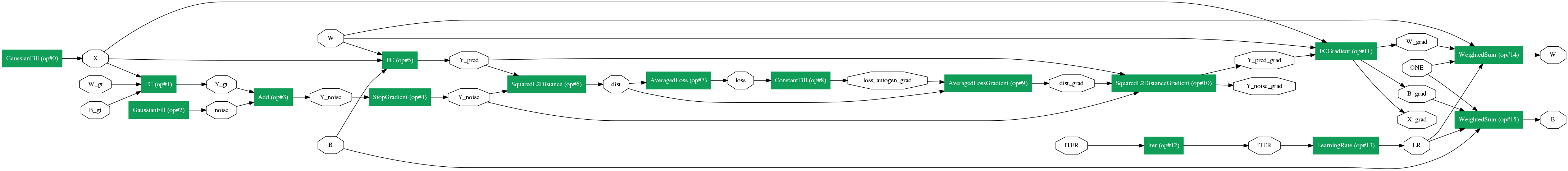

Now that we have created the networks ,let’s run them.

workspace.RunNetOnce(init_net)workspace.CreateNet(train_net)

看一下参数

print("Before training, W is: {}".format(workspace.FetchBlob("W")))print("Before training, B is: {}".format(workspace.FetchBlob("B")))

Results：

Before training, W is: [[-0.77634162 -0.88467366]]Before training, B is: [ 0.]

for i in range(100):    workspace.RunNet(train_net.Proto().name)

看一下学习后的参数

print("After training, W is: {}".format(workspace.FetchBlob("W")))print("After training, B is: {}".format(workspace.FetchBlob("B")))print("Ground truth W is: {}".format(workspace.FetchBlob("W_gt")))print("Ground truth B is: {}".format(workspace.FetchBlob("B_gt")))

Results:

After training, W is: [[ 1.95769441  1.47348857]]After training, B is: [ 0.45236012]Ground truth W is: [[ 2.   1.5]]Ground truth B is: [ 0.5]

看起来很简单吧？ 我们来仔细看看参数更新在训练步骤中的进展情况。 为此，让我们重新初始化参数，并查看步骤中参数的更改。 记住我们可以随时从工作区获取Blob。

workspace.RunNetOnce(init_net)w_history=[]b_history=[]for i in range(50):    workspace.RunNet(train_net.Proto().name)    w_history.append(workspace.FetchBlob("W"))    b_history.append(workspace.FetchBlob("B"))w_history=np.vstack(w_history)b_history = np.vstack(b_history)pyplot.plot(w_history[:, 0], w_history[:, 1], 'r')pyplot.axis('equal')pyplot.xlabel('w_0')pyplot.ylabel('w_1')pyplot.grid(True)pyplot.figure()pyplot.plot(b_history)pyplot.xlabel('iter')pyplot.ylabel('b')pyplot.grid(True)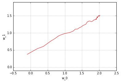

您可以观察随机梯度下降的非常典型的行为：由于噪音在整个训练过程中波动很大。 尝试多次运行上述ipython笔记本程序块 - 您将看到不同的初始化和不同噪音对结果的影响。

这只是一牛刀小试，在MNIST例子中展示真正的神经网络训练。