CNTK API文档翻译(9)——使用自编码器压缩MNIST数据

在本期教程之前需要先完成第四期教程。

介绍

本教程介绍自编码器的基础。自编码器是一种用于高效编码的无监督学习人工神经网络，换句话说，自编码器用于通过机器学习学来的算法而不是人写的算法进行有损数据压缩。由此而来，使用自编码器编码的目的是训练出一套数据表示方法来编码或者说表述一个数据集，经常被用于数据降维。

自编码器非常依赖于不同的数据，他们和传统的编码/解码器比如JPEG，MPEG等非常不同，没有一个编码标准。由于是有损压缩，因此当一段数据被编码然后又解码回去，会有一部分信息丢失，所以自编码器基本不会真正用于数据压缩，缺在两大领域有奇效：去噪和数据降维。

自编码器一直默默无闻，直到科学家们发现他在无监督学习上大有可为。真正的无监督学习是完全不需要标记的，不过自编码器因为可以进行自对照，因此也被叫做自监督学习，也就是把输入数据当标记的机器学习。

目标

我们的目标是训练一个自编码器，把MNIST数据压缩成一个更小维度的矢量，然后再保存成图像。MNIST是由一些有点背景噪音的手写数字图像组成的。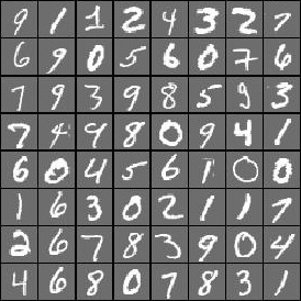

在本教程中，我们会使用MNIST数据来展示使用前馈神经网络编码和解码图像。我们会对比编码前的图像和经过编码解码之后的图像。我们会使用前馈神经网络构建简单自编码器和深度自编码器。更多的自编码器会在以后的教程中涉及到。

# Import the relevant modulesfrom __future__ import print_function # Use a function definition from future version (say 3.x from 2.7 interpreter)import matplotlib.pyplot as pltimport numpy as npimport osimport sys# Import CNTK import cntk as C

在下面的代码中，我们通过检查在CNTK内部定义的环境变量来选择正确的设备（GPU或者CPU）来运行代码，如果不检查的话，会使用CNTK的默认策略来使用最好的设备（如果GPU可用的话就使用GPU，否则使用CPU）

# Select the right target device when this notebook is being tested:if 'TEST_DEVICE' in os.environ:    if os.environ['TEST_DEVICE'] == 'cpu':        C.device.try_set_default_device(C.device.cpu())    else:        C.device.try_set_default_device(C.device.gpu(0))

我们设定了两种运行模式：

• 快速模式：isFast变量设置成True。这是我们的默认模式，在这个模式下我们会训练更少的次数，也会使用更少的数据，这个模式保证功能的正确性，但训练的结果还远远达不到可用的要求。
• 慢速模式：我们建议学习者在学习的时候试试将isFast变量设置成False，这会让学习者更加了解本教程的内容。

数据读取

在本部分我们将使用第四期下载的数据。数据格式如下：
|labels 0 0 0 1 0 0 0 0 0 0 |features 0 0 0 0 … (784 integers each representing a pixel gray level)

在本期教程中，我们使用代表像素值的数值串作为特征值。下面定义create_reader函数来读取训练数据和测试数据，代码中使用到了CTF（CNTK text-format） Deserializer，标签使用一位有效编码。

# Read a CTF formatted text (as mentioned above) using the CTF deserializer from a filedef create_reader(path, is_training, input_dim, num_label_classes):    return C.io.MinibatchSource(C.io.CTFDeserializer(path, C.io.StreamDefs(        labels_viz = C.io.StreamDef(field='labels', shape=num_label_classes, is_sparse=False),        features   = C.io.StreamDef(field='features', shape=input_dim, is_sparse=False)    )), randomize = is_training, max_sweeps = C.io.INFINITELY_REPEAT if is_training else 1)# Ensure the training and test data is generated and available for this tutorial.# We search in two locations in the toolkit for the cached MNIST data set.data_found = Falsefor data_dir in [os.path.join("..", "Examples", "Image", "DataSets", "MNIST"),                 os.path.join("data", "MNIST")]:    train_file = os.path.join(data_dir, "Train-28x28_cntk_text.txt")    test_file = os.path.join(data_dir, "Test-28x28_cntk_text.txt")    if os.path.isfile(train_file) and os.path.isfile(test_file):        data_found = True        breakif not data_found:    raise ValueError("Please generate the data by completing CNTK 103 Part A")print("Data directory is {0}".format(data_dir))

模型创建

我们首先假设用一个简单的全连接前馈神经网络来当作编码器和解码器（如下图）。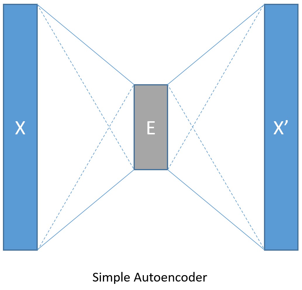

输入数据使用MNIST的手写数字图像，每个图像都是28×28像素。在本教程中，我们把每个图像都当做一个线性数组，里面的值就是这784个像素的像素值，所以输入值的大小应该是784。因为我们的目标是先编码然后解码，所以输出的大小应该跟输入的大小一样。我们将设定压缩后的数据大小是32。另外像素值范围是0到255，在输入时需要归一化成0到1之间。

input_dim = 784encoding_dim = 32output_dim = input_dimdef create_model(features):    with C.layers.default_options(init = C.glorot_uniform()):        # We scale the input pixels to 0-1 range        encode = C.layers.Dense(encoding_dim, activation = C.relu)(features/255.0)        decode = C.layers.Dense(input_dim, activation = C.sigmoid)(encode)    return decode

训练和测试

在以前的教程中，我们经常把训练和测试分成不同的小结，这期我们把他们合在一起，这种方式在以后的实际应用中也可以使用。

train_and_test函数主要执行了如下两个任务：

• 训练模型
• 用测试数据评估模型精度

在训练时：

设定了三个网络的输入值，分别是reader_train（数据读取器），model_func（模型函数）和label（标签）。在本教程中，我们展示了如何创建和使用自己的成本函数。如上文所述，我们需要归一化label函数，让他的输出值在0和1之间，方便我们使用C.classification_error来计算差值。
在CNTK提供的一系列训练器中，我们选择Adam训练器。

在测试时：

另外引入了reader_test（测试数据读取器），用来和通过模型生成的像素值对比。

def train_and_test(reader_train, reader_test, model_func):    ###############################################    # Training the model    ###############################################    # Instantiate the input and the label variables    input = C.input_variable(input_dim)    label = C.input_variable(input_dim)    # Create the model function    model = model_func(input)    # The labels for this network is same as the input MNIST image.    # Note: Inside the model we are scaling the input to 0-1 range    # Hence we rescale the label to the same range    # We show how one can use their custom loss function    # loss = -(y* log(p)+ (1-y) * log(1-p)) where p = model output and y = target    # We have normalized the input between 0-1. Hence we scale the target to same range    target = label/255.0     loss = -(target * C.log(model) + (1 - target) * C.log(1 - model))    label_error  = C.classification_error(model, target)    # training config    epoch_size = 30000        # 30000 samples is half the dataset size     minibatch_size = 64    num_sweeps_to_train_with = 5 if isFast else 100    num_samples_per_sweep = 60000    num_minibatches_to_train = (num_samples_per_sweep * num_sweeps_to_train_with) // minibatch_size    # Instantiate the trainer object to drive the model training    lr_per_sample = [0.00003]    lr_schedule = C.learning_rate_schedule(lr_per_sample, C.UnitType.sample, epoch_size)    # Momentum    momentum_as_time_constant = C.momentum_as_time_constant_schedule(700)    # We use a variant of the Adam optimizer which is known to work well on this dataset    # Feel free to try other optimizers from     # https://www.cntk.ai/pythondocs/cntk.learner.html#module-cntk.learner    learner = C.fsadagrad(model.parameters,                         lr=lr_schedule, momentum=momentum_as_time_constant)     # Instantiate the trainer    progress_printer = C.logging.ProgressPrinter(0)    trainer = C.Trainer(model, (loss, label_error), learner, progress_printer)    # Map the data streams to the input and labels.    # Note: for autoencoders input == label    input_map = {        input  : reader_train.streams.features,        label  : reader_train.streams.features    }     aggregate_metric = 0    for i in range(num_minibatches_to_train):        # Read a mini batch from the training data file        data = reader_train.next_minibatch(minibatch_size, input_map = input_map)        # Run the trainer on and perform model training        trainer.train_minibatch(data)        samples = trainer.previous_minibatch_sample_count        aggregate_metric += trainer.previous_minibatch_evaluation_average * samples    train_error = (aggregate_metric*100.0) / (trainer.total_number_of_samples_seen)    print("Average training error: {0:0.2f}%".format(train_error))    #############################################################################    # Testing the model    # Note: we use a test file reader to read data different from a training data    #############################################################################    # Test data for trained model    test_minibatch_size = 32    num_samples = 10000    num_minibatches_to_test = num_samples / test_minibatch_size    test_result = 0.0    # Test error metric calculation    metric_numer    = 0    metric_denom    = 0    test_input_map = {        input  : reader_test.streams.features,        label  : reader_test.streams.features    }    for i in range(0, int(num_minibatches_to_test)):        # We are loading test data in batches specified by test_minibatch_size        # Each data point in the minibatch is a MNIST digit image of 784 dimensions         # with one pixel per dimension that we will encode / decode with the         # trained model.        data = reader_test.next_minibatch(test_minibatch_size,                                       input_map = test_input_map)        # Specify the mapping of input variables in the model to actual        # minibatch data to be tested with        eval_error = trainer.test_minibatch(data)        # minibatch data to be trained with        metric_numer += np.abs(eval_error * test_minibatch_size)        metric_denom += test_minibatch_size    # Average of evaluation errors of all test minibatches    test_error = (metric_numer*100.0) / (metric_denom)     print("Average test error: {0:0.2f}%".format(test_error))    return model, train_error, test_error

我们先准备两个数据读取器，然后训练：

num_label_classes = 10reader_train = create_reader(train_file, True, input_dim, num_label_classes)reader_test = create_reader(test_file, False, input_dim, num_label_classes)model, simple_ae_train_error, simple_ae_test_error = train_and_test(reader_train, reader_test, model_func = create_model )

输出值：

 average      since    average      since      examples    loss       last     metric       last               ------------------------------------------------------Learning rate per sample: 3e-05      544        544      0.947      0.947            64      544        544      0.931      0.923           192      543        543      0.921      0.913           448      542        541      0.924      0.927           960      537        532      0.924      0.924          1984      493        451      0.821      0.721          4032      383        275      0.639       0.46          8128      303        223      0.524      0.409         16320      251        199      0.396      0.268         32704      209        168      0.281      0.167         65472      174        139      0.194      0.107        131008      144        113      0.125     0.0554        262080Average training error: 11.33%Average test error: 3.12%

可视化简单自编码器的结果

# Read some data to run the evalnum_label_classes = 10reader_eval = create_reader(test_file, False, input_dim, num_label_classes)eval_minibatch_size = 50eval_input_map = { input  : reader_eval.streams.features }    eval_data = reader_eval.next_minibatch(eval_minibatch_size,                                  input_map = eval_input_map)img_data = eval_data[input].asarray()# Select a random imagenp.random.seed(0) idx = np.random.choice(eval_minibatch_size)orig_image = img_data[idx,:,:]decoded_image = model.eval(orig_image)[0]*255# Print image statisticsdef print_image_stats(img, text):    print(text)    print("Max: {0:.2f}, Median: {1:.2f}, Mean: {2:.2f}, Min: {3:.2f}".format(np.max(img),np.median(img),np.mean(img),np.min(img))) # Print original imageprint_image_stats(orig_image, "Original image statistics:")# Print decoded imageprint_image_stats(decoded_image, "Decoded image statistics:")

输出结果

Original image statistics:Max: 255.00, Median: 0.00, Mean: 24.07, Min: 0.00Decoded image statistics:Max: 249.56, Median: 0.58, Mean: 27.02, Min: 0.00

然后我们把原始图片和经过编码解码之后的图片展示出来，理论上他们看起来应该挺像的。

# Define a helper function to plot a pair of imagesdef plot_image_pair(img1, text1, img2, text2):    fig, axes = plt.subplots(nrows=1, ncols=2, figsize=(6, 6))    axes[0].imshow(img1, cmap="gray")    axes[0].set_title(text1)    axes[0].axis("off")    axes[1].imshow(img2, cmap="gray")    axes[1].set_title(text2)    axes[1].axis("off")# Plot the original and the decoded imageimg1 = orig_image.reshape(28,28)text1 = 'Original image'img2 = decoded_image.reshape(28,28)text2 = 'Decoded image'plot_image_pair(img1, text1, img2, text2)

深度自解码器

我们当然没必要把编码和解码器限制在一层，我们可以使用多个全连接层来创建深度自解码器。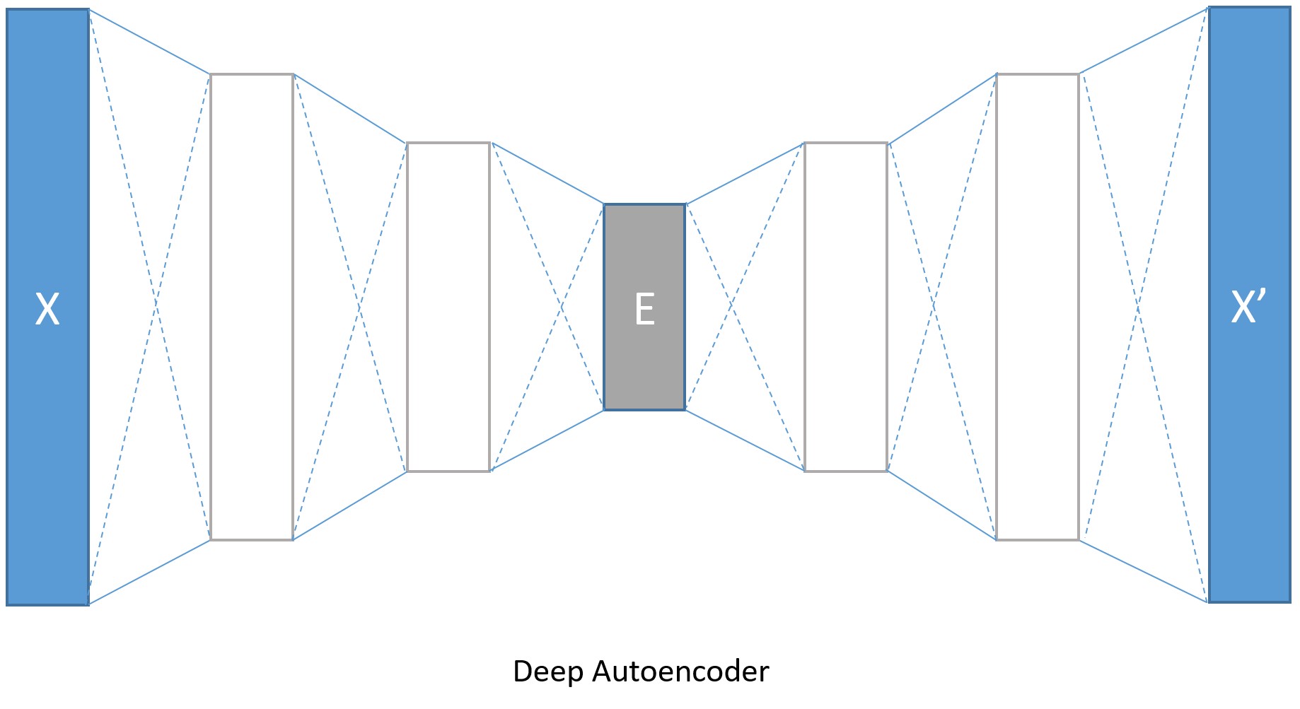

编码层的大小分别是128，64，32，与之对应，解码层就分别是64，128，784。转换模型参数的增加会带来更低的错误率，当然也会带来训练时间和内存占用增多的代价。如果我们在训练深度编码器时将isFast设置成False，训练就会进行更多轮，我们将得到更低的错误率，最后解码的图像边缘也会更清晰。

input_dim = 784encoding_dims = [128,64,32]decoding_dims = [64,128]encoded_model = Nonedef create_deep_model(features):    with C.layers.default_options(init = C.layers.glorot_uniform()):        encode = C.element_times(C.constant(1.0/255.0), features)        for encoding_dim in encoding_dims:            encode = C.layers.Dense(encoding_dim, activation = C.relu)(encode)        global encoded_model        encoded_model= encode        decode = encode        for decoding_dim in decoding_dims:            decode = C.layers.Dense(decoding_dim, activation = C.relu)(decode)        decode = C.layers.Dense(input_dim, activation = C.sigmoid)(decode)        return decodenum_label_classes = 10reader_train = create_reader(train_file, True, input_dim, num_label_classes)reader_test = create_reader(test_file, False, input_dim, num_label_classes)model, deep_ae_train_error, deep_ae_test_error = train_and_test(reader_train, reader_test, model_func = create_deep_model)

结果：

 average      since    average      since      examples    loss       last     metric       last               ------------------------------------------------------Learning rate per sample: 3e-05      543        543      0.928      0.928            64      543        543      0.925      0.923           192      543        543      0.907      0.894           448      542        541      0.891      0.877           960      527        513      0.768      0.652          1984      411        299       0.63      0.496          4032      313        217      0.547      0.466          8128      260        206      0.476      0.405         16320      220        181      0.377      0.278         32704      183        146      0.275      0.174         65472      150        118      0.185     0.0947        131008      125        100      0.119     0.0531        262080Average training error: 10.90%Average test error: 3.37%

可视化深度自编码器的结果

# Run the same image as the simple autoencoder through the deep encoderorig_image = img_data[idx,:,:]decoded_image = model.eval(orig_image)[0]*255# Print image statisticsdef print_image_stats(img, text):    print(text)    print("Max: {0:.2f}, Median: {1:.2f}, Mean: {2:.2f}, Min: {3:.2f}".format(np.max(img),np.median(img),np.mean(img),np.min(img))) # Print original imageprint_image_stats(orig_image, "Original image statistics:")# Print decoded imageprint_image_stats(decoded_image, "Decoded image statistics:")

然后我们把原始图片和经过编码解码之后的图片展示出来，理论上他们看起来应该挺像的

# Plot the original and the decoded imageimg1 = orig_image.reshape(28,28)text1 = 'Original image'img2 = decoded_image.reshape(28,28)text2 = 'Decoded image'plot_image_pair(img1, text1, img2, text2)

我们上面展示了怎样对一个输入数据编码和解码。接下来我们会展示输入数据之间的比较和如何从输入数据中提取编码之后的数据。t-SNE可能是将将高维数据可视化成2D的最好方法，但是使用t-SNE时通常需要相对低维的数据，所以将数据使用自编码器编码成较低维度（比如32维）的数据，然后使用t-SNE映射成2D是一个比较好的方法。

所以接下来我们将使用深度自编码器的输出结果做如下工作：

• 压缩/编码两个图片
• 展示我们如何能得到两个图片编码之后的数据。

首先我们需要读取一些图片和他们的标记

# Read some data to run get the image data and the corresponding labelsnum_label_classes = 10reader_viz = create_reader(test_file, False, input_dim, num_label_classes)image = C.input_variable(input_dim)image_label = C.input_variable(num_label_classes)viz_minibatch_size = 50viz_input_map = {     image  : reader_viz.streams.features,     image_label  : reader_viz.streams.labels_viz }    viz_data = reader_eval.next_minibatch(viz_minibatch_size,                                  input_map = viz_input_map)img_data   = viz_data[image].asarray()imglabel_raw = viz_data[image_label].asarray()# Map the image labels into indices in minibatch arrayimg_labels = [np.argmax(imglabel_raw[i,:,:]) for i in range(0, imglabel_raw.shape[0])]       from collections import defaultdictlabel_dict=defaultdict(list)for img_idx, img_label, in enumerate(img_labels):    label_dict[img_label].append(img_idx)        # Print indices corresponding to 3 digitsrandIdx = [1, 3, 9]for i in randIdx:    print("{0}: {1}".format(i, label_dict[i]))

我们将使用scipy计算两张图片的余弦距离。

from scipy import spatialdef image_pair_cosine_distance(img1, img2):    if img1.size != img2.size:        raise ValueError("Two images need to be of same dimension")    return 1 - spatial.distance.cosine(img1, img2)# Let s compute the distance between two images of the same numberdigit_of_interest = 6digit_index_list = label_dict[digit_of_interest]if len(digit_index_list) < 2:    print("Need at least two images to compare")else:    imgA = img_data[digit_index_list[0],:,:][0]     imgB = img_data[digit_index_list[1],:,:][0]    # Print distance between original image    imgA_B_dist = image_pair_cosine_distance(imgA, imgB)    print("Distance between two original image: {0:.3f}".format(imgA_B_dist))    # Plot the two images    img1 = imgA.reshape(28,28)    text1 = 'Original image 1'    img2 = imgB.reshape(28,28)    text2 = 'Original image 2'    plot_image_pair(img1, text1, img2, text2)    # Decode the encoded stream     imgA_decoded =  model.eval([imgA])[0]    imgB_decoded =  model.eval([imgB])   [0]        imgA_B_decoded_dist = image_pair_cosine_distance(imgA_decoded, imgB_decoded)    # Print distance between original image    print("Distance between two decoded image: {0:.3f}".format(imgA_B_decoded_dist))    # Plot the two images    # Plot the original and the decoded image    img1 = imgA_decoded.reshape(28,28)    text1 = 'Decoded image 1'    img2 = imgB_decoded.reshape(28,28)    text2 = 'Decoded image 2'    plot_image_pair(img1, text1, img2, text2)

注：上余弦距离如果是1表示两个数据非常相似，余弦距离是0表示一点都不相似。

任务2是如何获取一个图片编码之后的矢量数据。也就是要求在网络示意图中标有E的部分。

imgA = img_data[digit_index_list[0],:,:][0] imgA_encoded =  encoded_model.eval([imgA])print("Length of the original image is {0:3d} and the encoded image is {1:3d}".format(len(imgA),len(imgA_encoded[0])))print("\nThe encoded image: ")print(imgA_encoded[0])

输出：

Length of the original image is 784 and the encoded image is  32The encoded image: [  0.          22.22325325   3.9777317   13.26123905   9.97513866   0.  13.37649727   6.18241978   5.78068304  12.50789165  20.11767769   9.77285862   0.          14.75064278  17.07588768   0.           3.6076715   8.29384613  20.11726952  15.80433846   3.4400022    0.           0.  14.63469696   3.61723995  15.29668236  10.98176098   7.29611969  16.65932465   9.66042233   5.93092394   0.        ]

我们来比较一下不同数字之间的余弦距离

digitA = 3digitB = 8digitA_index = label_dict[digitA]digitB_index = label_dict[digitB]imgA = img_data[digitA_index[0],:,:][0] imgB = img_data[digitB_index[0],:,:][0]# Print distance between original imageimgA_B_dist = image_pair_cosine_distance(imgA, imgB)print("Distance between two original image: {0:.3f}".format(imgA_B_dist))# Plot the two imagesimg1 = imgA.reshape(28,28)text1 = 'Original image 1'img2 = imgB.reshape(28,28)text2 = 'Original image 2'plot_image_pair(img1, text1, img2, text2)# Decode the encoded stream imgA_decoded =  model.eval([imgA])[0]imgB_decoded =  model.eval([imgB])[0]    imgA_B_decoded_dist = image_pair_cosine_distance(imgA_decoded, imgB_decoded)#Print distance between original imageprint("Distance between two decoded image: {0:.3f}".format(imgA_B_decoded_dist))# Plot the original and the decoded imageimg1 = imgA_decoded.reshape(28,28)text1 = 'Decoded image 1'img2 = imgB_decoded.reshape(28,28)text2 = 'Decoded image 2'plot_image_pair(img1, text1, img2, text2)

欢迎扫码关注我的微信公众号获取最新文章