Kalman filter Intro - wiki

来源：互联网发布：阿里云自建ss 编辑：程序博客网时间：2024/05/04 09:49

https://en.wikipedia.org/wiki/Kalman_filter

Underlying dynamic system model[edit]

This section requires expansion. (August 2011)

The Kalman filters are based on linear dynamic systems discretized in the time domain. They are modelled on aMarkov chain built on linear operators perturbed by errors that may include Gaussian noise. The state of the system is represented as a vector of real numbers. At each discrete time increment, a linear operator is applied to the state to generate the new state, with some noise mixed in, and optionally some information from the controls on the system if they are known. Then, another linear operator mixed with more noise generates the observed outputs from the true ("hidden") state. The Kalman filter may be regarded as analogous to the hidden Markov model, with the key difference that the hidden state variables take values in a continuous space (as opposed to a discrete state space as in the hidden Markov model). There is a strong duality between the equations of the Kalman Filter and those of the hidden Markov model. A review of this and other models is given in Roweis andGhahramani (1999)^[11] and Hamilton (1994), Chapter 13.^[12]

In order to use the Kalman filter to estimate the internal state of a process given only a sequence of noisy observations, one must model the process in accordance with the framework of the Kalman filter. This means specifying the following matrices:F_k, the state-transition model;H_k, the observation model;Q_k, the covariance of the process noise;R_k, the covariance of the observation noise; and sometimesB_k, the control-input model, for each time-step,k, as described below.

Model underlying the Kalman filter. Squares represent matrices. Ellipses representmultivariate normal distributions (with the mean and covariance matrix enclosed). Unenclosed values arevectors. In the simple case, the various matrices are constant with time, and thus the subscripts are dropped, but the Kalman filter allows any of them to change each time step.

The Kalman filter model assumes the true state at time k is evolved from the state at (k − 1) according to

\mathbf{x}_{k} = \mathbf{F}_{k} \mathbf{x}_{k-1} + \mathbf{B}_{k} \mathbf{u}_{k} + \mathbf{w}_{k}

where

F_k is the state transition model which is applied to the previous statex_k−1;
B_k is the control-input model which is applied to the control vectoru_k;
w_k is the process noise which is assumed to be drawn from a zero meanmultivariate normal distribution with covariance Q_k.

\mathbf{w}_k \sim N(0, \mathbf{Q}_k)

At time k an observation (or measurement) z_k of the true statex_k is made according to

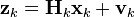
\mathbf{z}_k = \mathbf{H}_{k} \mathbf{x}_k + \mathbf{v}_k

where H_k is the observation model which maps the true state space into the observed space andv_k is the observation noise which is assumed to be zero mean Gaussianwhite noise with covariance R_k.

\mathbf{v}_k \sim N(0, \mathbf{R}_k)

The initial state, and the noise vectors at each step {x₀,w₁, …, w_k,v₁ … v_k} are all assumed to be mutuallyindependent.

Many real dynamical systems do not exactly fit this model. In fact, unmodelled dynamics can seriously degrade the filter performance, even when it was supposed to work with unknown stochastic signals as inputs. The reason for this is that the effect of unmodelled dynamics depends on the input, and, therefore, can bring the estimation algorithm to instability (it diverges). On the other hand, independent white noise signals will not make the algorithm diverge. The problem of separating between measurement noise and unmodelled dynamics is a difficult one and is treated in control theory under the framework ofrobust control.^[13]^[14]

Details[edit]

The Kalman filter is a recursive estimator. This means that only the estimated state from the previous time step and the current measurement are needed to compute the estimate for the current state. In contrast to batch estimation techniques, no history of observations and/or estimates is required. In what follows, the notation $\hat{\mathbf{x}}_{n\mid m}$ represents the estimate of $\mathbf{x}$ at timen given observations up to, and including at time m ≤ n.

The state of the filter is represented by two variables:

$\hat{\mathbf{x}}_{k\mid k}$ , thea posteriori state estimate at timek given observations up to and including at time k;
$\mathbf{P}_{k\mid k}$ , thea posteriori error covariance matrix (a measure of the estimated accuracy of the state estimate).

The Kalman filter can be written as a single equation, however it is most often conceptualized as two distinct phases: "Predict" and "Update". The predict phase uses the state estimate from the previous timestep to produce an estimate of the state at the current timestep. This predicted state estimate is also known as the a priori state estimate because, although it is an estimate of the state at the current timestep, it does not include observation information from the current timestep. In the update phase, the current a priori prediction is combined with current observation information to refine the state estimate. This improved estimate is termed thea posteriori state estimate.

Typically, the two phases alternate, with the prediction advancing the state until the next scheduled observation, and the update incorporating the observation. However, this is not necessary; if an observation is unavailable for some reason, the update may be skipped and multiple prediction steps performed. Likewise, if multiple independent observations are available at the same time, multiple update steps may be performed (typically with different observation matricesH_k).^[15]^[16]

Predict[edit]

Predicted (a priori) state estimate

\hat{\mathbf{x}}_{k\mid k-1} = \mathbf{F}_{k}\hat{\mathbf{x}}_{k-1\mid k-1} + \mathbf{B}_{k} \mathbf{u}_{k}

Predicted (a priori) estimate covariance

\mathbf{P}_{k\mid k-1} = \mathbf{F}_{k} \mathbf{P}_{k-1\mid k-1} \mathbf{F}_{k}^{\text{T}} + \mathbf{Q}_{k}

Update[edit]

Innovation or measurement residual

\tilde{\mathbf{y}}_k = \mathbf{z}_k - \mathbf{H}_k\hat{\mathbf{x}}_{k\mid k-1}

Innovation (or residual) covariance

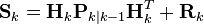\mathbf{S}_k = \mathbf{H}_k \mathbf{P}_{k\mid k-1} \mathbf{H}_k^T + \mathbf{R}_k

Optimal Kalman gain

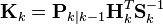\mathbf{K}_k = \mathbf{P}_{k\mid k-1}\mathbf{H}_k^T \mathbf{S}_k^{-1}

Updated (a posteriori) state estimate

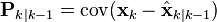
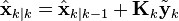\hat{\mathbf{x}}_{k\mid k} = \hat{\mathbf{x}}_{k\mid k-1} + \mathbf{K}_k\tilde{\mathbf{y}}_k

Updated (a posteriori) estimate covariance

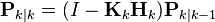
\mathbf{P}_{k|k} = (I - \mathbf{K}_k \mathbf{H}_k) \mathbf{P}_{k|k-1}

The formula for the updated estimate covariance above is only valid for the optimal Kalman gain. Usage of other gain values require a more complex formula found in thederivations section.

Invariants[edit]

If the model is accurate, and the values for $\hat{\mathbf{x}}_{0\mid 0}$ and $\mathbf{P}_{0\mid 0}$ accurately reflect the distribution of the initial state values, then the following invariants are preserved: (all estimates have a mean error of zero)

$\mathbf{E}[\mathbf{x}_k - \hat{\mathbf{x}}_{k\mid k}] = \textrm{E}[\mathbf{x}_k - \hat{\mathbf{x}}_{k\mid k-1}] = 0$
$\textrm{E}[\tilde{\mathbf{y}}_k] = 0$

where $\textrm{E}[\xi]$ is theexpected value of $\xi$ , and covariance matrices accurately reflect the covariance of estimates

$\mathbf{P}_{k\mid k} = \mathrm{cov}(\mathbf{x}_k - \hat{\mathbf{x}}_{k\mid k})$
$\mathbf{P}_{k\mid k-1} = \mathrm{cov}(\mathbf{x}_k - \hat{\mathbf{x}}_{k\mid k-1})$
$\mathbf{S}_{k} = \mathrm{cov}(\tilde{\mathbf{y}}_k)$

Optimality and performance[edit]

It follows from theory that the Kalman filter is optimal in cases where a) the model perfectly matches the real system, b) the entering noise is white and c) the covariances of the noise are exactly known. Several methods for the noise covariance estimation have been proposed during past decades, including ALS, mentioned in the previous paragraph. After the covariances are estimated, it is useful to evaluate the performance of the filter, i.e. whether it is possible to improve the state estimation quality. If the Kalman filter works optimally, the innovation sequence (the output prediction error) is a white noise, therefore the whiteness property of the innovations measures filter performance. Several different methods can be used for this purpose.^[17]

Example application, technical[edit]

Black: truth, green: filtered process, red: observations

Consider a truck on frictionless, straight rails. Initially the truck is stationary at position 0, but it is buffeted this way and that by random uncontrolled forces. We measure the position of the truck every Δt seconds, but these measurements are imprecise; we want to maintain a model of where the truck is and what its velocity is. We show here how we derive the model from which we create our Kalman filter.

Since $\mathbf F, \mathbf H, \mathbf R, \mathbf Q$ are constant, their time indices are dropped.

The position and velocity of the truck are described by the linear state space

\mathbf{x}_{k} = \begin{bmatrix} x \\ \dot{x} \end{bmatrix}

where $\dot{x}$ is the velocity, that is, the derivative of position with respect to time.

We assume that between the (k − 1) and k timestep uncontrolled forces cause a constant acceleration ofa_k that is normally distributed, with mean 0 and standard deviation σ_a. FromNewton's laws of motion we conclude that

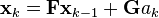
\mathbf{x}_{k} = \mathbf{F} \mathbf{x}_{k-1} + \mathbf{G}a_{k}

(note that there is no $\mathbf{B}u$ term since we have no known control inputs. Instead, we assume thata_k is the effect of an unknown input and $\mathbf{G}$ applies that effect to the state vector) where

\mathbf{F} = \begin{bmatrix} 1 & \Delta t \\ 0 & 1 \end{bmatrix}

and

\mathbf{G} = \begin{bmatrix} \frac{\Delta t^2}{2} \\[6pt] \Delta t \end{bmatrix}

so that

\mathbf{x}_{k} = \mathbf{F} \mathbf{x}_{k-1} + \mathbf{w}_{k}

where $\mathbf{w}_{k} \sim N(0, \mathbf{Q})$ and

\mathbf{Q}=\mathbf{G}\mathbf{G}^{\text{T}}\sigma_a^2 =\begin{bmatrix} \frac{\Delta t^4}{4} & \frac{\Delta t^3}{2} \\[6pt] \frac{\Delta t^3}{2} & \Delta t^2 \end{bmatrix}\sigma_a^2.

At each time step, a noisy measurement of the true position of the truck is made. Let us suppose the measurement noisev_k is also normally distributed, with mean 0 and standard deviationσ_z.

\mathbf{z}_{k} = \mathbf{H x}_{k} + \mathbf{v}_{k}

where

\mathbf{H} = \begin{bmatrix} 1 & 0 \end{bmatrix}

and

\mathbf{R} = \textrm{E}[\mathbf{v}_k \mathbf{v}_k^{\text{T}}] = \begin{bmatrix} \sigma_z^2 \end{bmatrix}

We know the initial starting state of the truck with perfect precision, so we initialize

\hat{\mathbf{x}}_{0\mid 0} = \begin{bmatrix} 0 \\ 0 \end{bmatrix}

and to tell the filter that we know the exact position and velocity, we give it a zero covariance matrix:

\mathbf{P}_{0\mid 0} = \begin{bmatrix} 0 & 0 \\ 0 & 0 \end{bmatrix}

If the initial position and velocity are not known perfectly the covariance matrix should be initialized with a suitably large number, sayL, on its diagonal.

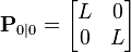
\mathbf{P}_{0\mid 0} = \begin{bmatrix} L & 0 \\ 0 & L \end{bmatrix}

The filter will then prefer the information from the first measurements over the information already in the model.

Derivations[edit]

This section needs additional citations forverification. Please help improve this article by adding citations to reliable sources. Unsourced material may be challenged and removed.(December 2010)

Deriving thea posteriori estimate covariance matrix[edit]

Starting with our invariant on the error covariance P_k | k as above

\mathbf{P}_{k\mid k} = \mathrm{cov}(\mathbf{x}_{k} - \hat{\mathbf{x}}_{k\mid k})

substitute in the definition of $\hat{\mathbf{x}}_{k\mid k}$

\mathbf{P}_{k\mid k} = \textrm{cov}(\mathbf{x}_{k} - (\hat{\mathbf{x}}_{k\mid k-1} + \mathbf{K}_k\tilde{\mathbf{y}}_{k}))

and substitute $\tilde{\mathbf{y}}_k$

\mathbf{P}_{k\mid k} = \textrm{cov}(\mathbf{x}_{k} - (\hat{\mathbf{x}}_{k\mid k-1} + \mathbf{K}_k(\mathbf{z}_k - \mathbf{H}_k\hat{\mathbf{x}}_{k\mid k-1})))

and $\mathbf{z}_{k}$

\mathbf{P}_{k\mid k} = \textrm{cov}(\mathbf{x}_{k} - (\hat{\mathbf{x}}_{k\mid k-1} + \mathbf{K}_k(\mathbf{H}_k\mathbf{x}_k + \mathbf{v}_k - \mathbf{H}_k\hat{\mathbf{x}}_{k\mid k-1})))

and by collecting the error vectors we get

\mathbf{P}_{k|k} = \textrm{cov}((I - \mathbf{K}_k \mathbf{H}_{k})(\mathbf{x}_k - \hat{\mathbf{x}}_{k\mid k-1}) - \mathbf{K}_k \mathbf{v}_k )

Since the measurement error v_k is uncorrelated with the other terms, this becomes

\mathbf{P}_{k|k} = \textrm{cov}((I - \mathbf{K}_k \mathbf{H}_{k})(\mathbf{x}_k - \hat{\mathbf{x}}_{k\mid k-1})) + \textrm{cov}(\mathbf{K}_k \mathbf{v}_k )

by the properties of vector covariance this becomes

\mathbf{P}_{k\mid k} = (I - \mathbf{K}_k \mathbf{H}_{k})\textrm{cov}(\mathbf{x}_k - \hat{\mathbf{x}}_{k\mid k-1})(I - \mathbf{K}_k \mathbf{H}_{k})^{\text{T}} + \mathbf{K}_k\textrm{cov}(\mathbf{v}_k )\mathbf{K}_k^{\text{T}}

which, using our invariant on P_k | k−1 and the definition ofR_k becomes

\mathbf{P}_{k\mid k} =(I - \mathbf{K}_k \mathbf{H}_{k}) \mathbf{P}_{k\mid k-1} (I - \mathbf{K}_k \mathbf{H}_{k})^\text{T} +\mathbf{K}_k \mathbf{R}_k \mathbf{K}_k^\text{T}

This formula (sometimes known as the "Joseph form" of the covariance update equation) is valid for any value ofK_k. It turns out that ifK_k is the optimal Kalman gain, this can be simplified further as shown below.

Kalman gain derivation[edit]

The Kalman filter is a minimum mean-square error estimator. The error in the a posteriori state estimation is

\mathbf{x}_{k} - \hat{\mathbf{x}}_{k\mid k}

We seek to minimize the expected value of the square of the magnitude of this vector, $\textrm{E}[\|\mathbf{x}_{k} - \hat{\mathbf{x}}_{k|k}\|^2]$ . This is equivalent to minimizing thetrace of the a posteriori estimate covariance matrix $\mathbf{P}_{k|k}$ . By expanding out the terms in the equation above and collecting, we get:

\begin{align}\mathbf{P}_{k\mid k} & = \mathbf{P}_{k\mid k-1} - \mathbf{K}_k \mathbf{H}_k \mathbf{P}_{k\mid k-1} - \mathbf{P}_{k\mid k-1} \mathbf{H}_k^\text{T} \mathbf{K}_k^\text{T} + \mathbf{K}_k (\mathbf{H}_k \mathbf{P}_{k\mid k-1} \mathbf{H}_k^\text{T} + \mathbf{R}_k) \mathbf{K}_k^\text{T} \\[6pt]& = \mathbf{P}_{k\mid k-1} - \mathbf{K}_k \mathbf{H}_k \mathbf{P}_{k\mid k-1} - \mathbf{P}_{k\mid k-1} \mathbf{H}_k^\text{T} \mathbf{K}_k^\text{T} + \mathbf{K}_k \mathbf{S}_k\mathbf{K}_k^\text{T}\end{align}

The trace is minimized when its matrix derivative with respect to the gain matrix is zero. Using the gradient matrix rules and the symmetry of the matrices involved we find that

\frac{\partial \; \mathrm{tr}(\mathbf{P}_{k\mid k})}{\partial \;\mathbf{K}_k} = -2 (\mathbf{H}_k \mathbf{P}_{k\mid k-1})^\text{T} + 2 \mathbf{K}_k \mathbf{S}_k = 0.

Solving this for K_k yields the Kalman gain:

\mathbf{K}_k \mathbf{S}_k = (\mathbf{H}_k \mathbf{P}_{k\mid k-1})^\text{T} = \mathbf{P}_{k\mid k-1} \mathbf{H}_k^\text{T}

\mathbf{K}_{k} = \mathbf{P}_{k\mid k-1} \mathbf{H}_k^\text{T} \mathbf{S}_k^{-1}

This gain, which is known as the optimal Kalman gain, is the one that yieldsMMSE estimates when used.

Simplification of thea posteriori error covariance formula[edit]

The formula used to calculate the a posteriori error covariance can be simplified when the Kalman gain equals the optimal value derived above. Multiplying both sides of our Kalman gain formula on the right byS_kK_k^T, it follows that

\mathbf{K}_k \mathbf{S}_k \mathbf{K}_k^\mathrm{T} = \mathbf{P}_{k\mid k-1} \mathbf{H}_k^\mathrm{T} \mathbf{K}_k^\mathrm{T}

Referring back to our expanded formula for the a posteriori error covariance,

\mathbf{P}_{k\mid k} = \mathbf{P}_{k\mid k-1} - \mathbf{K}_k \mathbf{H}_k \mathbf{P}_{k\mid k-1} - \mathbf{P}_{k\mid k-1} \mathbf{H}_k^\mathrm{T} \mathbf{K}_k^\mathrm{T} + \mathbf{K}_k \mathbf{S}_k \mathbf{K}_k^\mathrm{T}

we find the last two terms cancel out, giving

\mathbf{P}_{k\mid k} = \mathbf{P}_{k\mid k-1} - \mathbf{K}_k \mathbf{H}_k \mathbf{P}_{k\mid k-1} = (I - \mathbf{K}_{k} \mathbf{H}_{k}) \mathbf{P}_{k\mid k-1}.

This formula is computationally cheaper and thus nearly always used in practice, but is only correct for the optimal gain. If arithmetic precision is unusually low causing problems withnumerical stability, or if a non-optimal Kalman gain is deliberately used, this simplification cannot be applied; thea posteriori error covariance formula as derived above (Joseph form) must be used.

0 0